Download
1 / 32
320 likes | 350 Views
A general introduction to Stata software for data handling, analysis, and creating graphs with syntax examples. Benefits, limitations, and tools for epidemiology.

E N D
Stata Introduction, Shortv2 Hein Stigum Presentation, data and programs at: http://folk.uio.no/heins/ courses Dec-19 H.S. H.S. 1
Stata introduction • General use • Interface and menu • Do-files and syntax • Data handling • Analysis • Descriptive • Graphs • Bivariate H.S.
Why Stata • Pro • Aimed at epidemiology • Many methods, growing • Graphics • Structured, Programmable • Coming soon to a course near you • Con • Memory>file size Dec-19 H.S. H.S. 3
Interface Stata 9 Dec-19 H.S. H.S. 5
Interface Stata 12 Do file Data edit H.S.
Menu Dec-19 H.S. H.S. 7
Do-file example New do-file: icon or Ctrl-9 Run: Mark, Ctrl-D Dec-19 H.S. H.S. 8
Syntax • Syntax [bysort varlist:] command [varlist] [if exp] [in range][, opts] • Examples • meanage • meanageif sex==1 • bysort sex: summarizeage • summarizeage,detail Dec-19 H.S. H.S. 9
Import data • Using SPSS 14.0-17.0 • Save as, Stata Version 8 SE Dec-19 H.S. H.S. 11
Use and save data • Open data • use “C:\Course\Myfile.dta”, clear • Describe • describe describe all variables • listx1 x2 in 1/20 list obs nr 1 to 20 • Save data • save “C:\Course\Myfile.dta” ,replace Dec-19 H.S. H.S. 12
Use data from web • webuse “file” use data from Stata homepage • webuse set “http://www.med.uio.no/forskning/doktorgrad-karriere/forskerutdanning/kurs/biostatistikk/mf9510-logistisk-regresjon-overlevelsesanalyse-cox/” set homepage • webuse “birth1” data for exercise 1 Dec-19 H.S. H.S. 13
Index generate index=0 replaceindex=1 if sex==1 & age<30 Young/Old generate old=(age>50) Serial numbers, lags generate id=_n generate age1=age[ _n-1] Generate, replace if age<. Dec-19 H.S. H.S. 14
Dates • From numeric to date ex: m=12, d=2, y=1987 generatebirth=mdy(m,d,y) formatbirth %td • From string to date ex: bstr=“01.12.1987” generatebirth=date(bstr,”DMY”) formatbirth %td Dec-19 H.S. H.S. 15
Missing • Obs!!! • Represented as ”.” • Missing values are large numbers • age>30 will include missing. • age>30 if age<. will not. • Test • replace age=0 if (age==.) • Remove • drop if age==. • Change • replace educ=. if educ==99 Dec-19 H.S. H.S. 16
Summarize variables Missing in tables Describe missing summarize id bullied sex tab bullied sex, missing misstable summarize bullied sex new command Dec-19 H.S. H.S. 17
Help • General • helpcommand • finditkeyword search Stata+net • Examples • help table • findit aflogit Dec-19 H.S. H.S. 18
Summing up • Use do files • Run: Mark, Ctrl-D • Syntax • command [varlist] [if exp] [in range] [, options] • Missing • age>30 if age<. • generateold=(age>50) if age<. • Help • help describe Dec-19 H.S. H.S. 19
Descriptive • Continuous summarize weight summarize weight, details fractiles ++ • Categorical tabulate bullied tabulate bullied,nolab show coding H.S.
Other descriptives tabstatmAge, stat( N min p50 mean max) by(parity) Dec-19 H.S. H.S. 22
Graphics H.S.
Twoway plots • Syntax • twoway (plot1, opts) (plot2, opts), opts • One plot • kdensity bw • scatter bw gest Dec-19 H.S. H.S. 24
twoway ( kdensitybwif sex==1, lcolor(blue) ) /// • ( kdensitybwif sex==2, lcolor(red ) ) Dec-19 H.S. H.S. 25
line fit scatter twoway(scatterbw gest) (fpfitcibw gest) (lfitbw gest) smooth with CI Dec-19 H.S. H.S. 26
Titles scatterbw gest, title("title") subtitle("subtitle") /// xtitle("xtitle") ytitle("ytitle") note("note") Dec-19 H.S. H.S. 27
2 independent samples Do boys and girls have the same mean birth weight? • twoway ( kdensity weight if sex==1, lcolor(blue) ) /// • ( kdensity weight if sex==2, lcolor(red) ) Equal means? Equal variance? Dec-19 H.S. H.S. 29
2 independent samples test ttest weight, by(sex) 2-sample T-test ttest weight, by(sex) unequal ttest w1 w2, paired Dec-19 H.S. H.S. 30
equal proportions? Crosstables Are boys bullied as much as girls? tabulate bullied sex, col chi2 nofreq Dec-19 H.S. H.S. 31
Summing up Descriptive summarizeweight tabulatesex Graphs twoway (plot1, opts) (plot2, opts), opts Bivariate ttest weight, by(sex) tabulatebullied sex, chi2 Dec-19 H.S. H.S. 32