Understanding Linear Trend Lines and Their Applications in Forecasting Sales
This guide details the concept of Linear Trend Lines in regression analysis, focusing on their role in forecasting dependent variables based on independent ones. Key components, such as the slope (b1) and y-intercept (b0), are explained using Excel tools. It also covers the coefficient of determination (R²), which measures how well the model fits the data, and the standard error of the estimate. An example demonstrates a linear regression model for predicting annual sales based on store size, showcasing practical applications of the trend analysis.

Understanding Linear Trend Lines and Their Applications in Forecasting Sales
E N D
Presentation Transcript
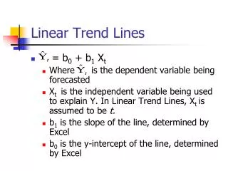
Linear Trend Lines • = b0 + b1Xt • Where is the dependent variable being forecasted • Xt is the independent variable being used to explain Y. In Linear Trend Lines, Xtis assumed to be t. • b1 is the slope of the line, determined by Excel • b0 is the y-intercept of the line, determined by Excel
Coefficient of Determination: R-square • Proportion of variation in Y around its mean that is accounted for by the regression model • 0 <= R2 <= 1 • Will always increase as add more independent variables into regression model. Use adjusted R2 to compare when more than one independent variable is used
Standard Error of the line: Se • The standard deviation of estimation errors • The measure of amount of scatter around the regression line • Can be used as a rough rule of thumb for predicting level of accuracy.
Excel’s Trend Function • =trend(known y-range, known x-range, new x) • Where known y-range are the cells that hold known values for the y variable • Where known x-range are the cells that hold known values for the x variable • Where new x is the cell or value for which the y variable is to be forecasted
Simple Linear Regression: Example You want to examine the linear dependency of the annual sales of produce stores on their size in square footage. Sample data for seven stores were obtained. Find the equation of the straight line that fits the data best. Annual Store Square Sales Feet ($1000) 1 1,726 3,681 2 1,542 3,395 3 2,816 6,653 4 5,555 9,543 5 1,292 3,318 6 2,208 5,563 7 1,313 3,760
Scatter Diagram: Example Excel Output
Equation for the Sample Regression Line: Example From Excel Printout:
Graph of the Sample Regression Line: Example Yi = 1636.415 +1.487Xi
Interpretation of Results: Example The slope of 1.487 means that for each increase of one unit in X, we predict the average of Y to increase by an estimated 1.487 units. The model estimates that for each increase of one square foot in the size of the store, the expected annual sales are predicted to increase by $1487.