Download
1 / 27
270 likes | 430 Views
Power-aware Topology Control in Wireless Ad Hoc Networks. David S. L. Wei Dept of Computer and Information Sciences Fordham University Bronx, New York. Joint work with. Szu-Chi Wang and Sy-Yen Kuo Dept of Electrical Engineering National Taiwan University Taipei, Taiwan. Introduction.

E N D
Power-aware Topology Control in Wireless Ad Hoc Networks David S. L. Wei Dept of Computer and Information Sciences Fordham University Bronx, New York Joint work with Szu-Chi Wang and Sy-Yen Kuo Dept of Electrical Engineering National Taiwan University Taipei, Taiwan
Introduction Wireless ad hoc networks are - Characterized by scarce resources - Prone to topology changes - Lack of physical infrastructure The flexibility and mobility of wireless ad hoc networks make them suitable for applications such as automated battlefields and disaster rescues
F F E D A C A C D E B B Introduction (cont.) • A wireless ad hoc network can be modeled by an undirected/directed graph G = (V, E) Power conservation has been widely used as a primary control parameter in the design of protocols for wireless ad hoc networks
F F E D A C A C D E B B E D A C A C D E F B F B Introduction (cont.)
Motivations Each node in a wireless ad hoc network can potentially change the network topology by adjusting its transmissionrange The primary goal of topology control is to design power-efficient algorithms that - Maintain network connectivity - Optimize performance metrics (network lifetime, throughput,…)
Preliminaries In the most common power-attenuation model - The transmission power between node u and v is denoted as - All receivers have the same power threshold for signal detection We assume that - Each mobile host has a low-power GPS receiver - Initially all the nodes are operated at full transmitter power ─ the resulted graph G is a unit-disk graph (denoted as UDG (V)) transmitter power t ||uv|| + rp(u,v) receiver power
Preliminaries (cont.) Hereinafter we use G to present a wireless ad hoc network - The edge weight is defined as w(u, v) = t||uv|| + rp(u,v) - We also call G the transmission graph A path from node u to node v is denoted as The total transmission power of this path is (u, v) = v0v1…vh-1vh where u = v0 and v = vh
Transmission Power Assignment A transmission power assignment on the vertices is a function f from V into real numbers Given a graph H = (V’, E’) , the transmission power assignment f is induced by H if for each node v V’, The total transmission power of f is defined as A transmission power assignment f is complete if the associated graph Gf is strongly connected
Minimum-Energy Path Given a communication graph H G, the minimum-energy path between node u and node v, denoted by Hmin(u, v), is a path whose total transmission power is the minimum among all paths that connect (u, v) in H Let pH(u, v) stand for p(Hmin(u, v)), the power stretch factor of H with respect to G is defined as
Related Works Our major work is to develop a localized topology control algorithm where each node makes a decision about its transmission power based on only its local information The two widely used energy conservation approaches in literature are to - Reduce the total transmission power - Reduce the power stretch factor However, these two approaches may offset each other
Related Works (cont.) The problem of finding a complete f whose total transmission power is the minimum among all of the complete assignments is called the min-total assignment problem The min-total assignment problem is NP-hard when the nodes are deployed in a d-dimensional space, d 2 The general structure of the minimum-power topology for rp 0 is still unknown
Basic Ideas The proposed algorithm is based on the following ideas - First construct a connected subgraph H = (V, E’) - Assure that the power stretch factor of H is bounded - The total transmission power is then minimized as much as possible We use the local information of each node to excise some links of G while still keeps the power stretch factor being bounded by a predetermined value cb
p3 p3 p2 p2 p1 p1 p4 p4 p5 p5 p6 p6 p7 p7 Our Localized Topology Control Algorithm The proposed algorithm consists of two phases - Phase I: Local shortest tree construction - Phase II: Path search replacement A simple illustrative example is shown below p3 p2 p1 p4 p5 p6 p7
Phase I of the Proposed Algorithm Definition 1 (Local Topology View) The local topology view of node u, LTV (u, k) = (V’, E’)), is a subgraph of G such that (1) viV’ if the hop distance between vi and u is no more than k (2) (vi, vj) E’ if both vi and vj belong to V’ Suppose that a subgraph of G is associated with a transmission power assignment f - For each node u, if link (u, v) satisfies w (u, v) = f (u) then (u, v) is called a critical link of u
Phase I of the Proposed Algorithm (cont.) Each node u individually applies Dijkstra’s algorithm to get the shortest-paths from the source u to the other nodes in LTV (u, 1) The local shortest path tree of node u (denoted by LSPT (u)) can thus be obtained DC (u) = {vV’ | h (LSPT (u), v) = 1}, where h (LSPT (u), v) is the height of a child node v in LSPT (u) Node u then deletes the edges {(u, w) | wDC (u)} The topology generated is denoted as GI
Phase II of the Proposed Algorithm For each node u, its transmission power could be further reduced by trying to eliminate the critical links that are replaceable with alternative paths For each critical link (u, v), node u tries to search another path that reaches node v based on LTV (u, k) - We call such path the replacing path of (u, v) - The entire replacing paths of node u is denoted as RP (u) The searching procedure is applying Dijkstra’s algorithm again on LTV (u, k)
Phase II of the Proposed Algorithm (cont.) If no such path exists or no replacing path has transmission power cb w (u, v) - The search process is ended - RP (u) is set as an empty list - ps (u) is set to 0 The priority of node u is a pair pri(u) = <ps(u), ID(u)> - pri(v1) = (ps(v1), ID1), pr (v2) = (ps(v2), ID2) - pri(v1) > pri(v2) if ps(v1) > ps(v2) (ps(v1) = ps(v2) ID1 < ID2) The above procedure for deciding RP (u) starts if node u has the highest priority in its k-hop neighborhood
Phase II of the Proposed Algorithm (cont.) After Phase I, each node deletes its uni-directional links and the resulting topology is denoted as GII The constructed topology after Phase II is denoted as GIII A simple heuristic for further decreasing the total transmission power is also proposed
Important Properties The minimum-energy path between any two nodes in G is preserved in GI The minimum-energy path between the two end nodes of each deleted link in GI is preserved in GII GII preserves the network connectivity of G is bounded by cb GIII preserves the network connectivity of G and has a bounded power stretch factor cb
Dealing with Mobility We also consider the case of modest movement of the nodes It would be extremely difficult for a topology control algorithm to even effectively guarantee network connectivity if network topology changes too fast As mentioned in previous works, node movement can be viewed as two events, namely nodeaddition and nodedeletion In our case, however, at the beginning of each beacon interval each node u should check if there is a change in transmission radius after deciding the new logical links
Performance Comparisons We compared the performance via extensive simulations We observe the following metrics of each constructed topology H - Total transmission power (denoted by tpc) - Power stretch mean (denoted by psm) - The maximum power stretch factor (denoted by maxpsf) - The variance of transmission power (denoted by var tp) - Average node degree (denoted by avg nd) - The maximum node degree (denoted by max nd)
Simulation Results The Performance Measurements with s = 1 The Performance Measurements with s = 3 The Performance Measurements with s = 5 The Performance Measurements with s = 7
Network topologies constructed by various algorithms I SMEN UDG GG AMST
Network topologies constructed by various algorithms II ESPT1 LMST ESPT2, cb = 1.5 ESPT2, cb = 2.0
Conclusions In this paper we develop a localized algorithm that requires only local information for constructing a logical topology on a given unit disk graph The topology constructed by our algorithm has several desired features such as bounded power stretch factor, low total power consumption, and small variance of transmission power The simulation results show that our algorithm outperforms others in terms of various important metrics
Future Research • Power-aware topology control • Topology control of ad-hoc networks in three-dimensional space • Secure topology control algorithm • Applications in overlay control for P2P communications