Download
1 / 23
230 likes | 356 Views
APECE-505 Intelligent System Engineering Low-level Processing Md. Atiqur Rahman Ahad. Reference books: - Computer Vision and Action Recognition, Md. Atiqur Rahman Ahad - Digital Image Processing, Gonzalez & Woods. Filtering – in spatial domain.

E N D
APECE-505 Intelligent System Engineering Low-level Processing Md. AtiqurRahmanAhad Reference books: - Computer Vision and Action Recognition, Md. Atiqur Rahman Ahad - Digital Image Processing, Gonzalez & Woods.
Filtering – in spatial domain — low-pass filters for smoothing/ blurring (demonstrates smooth areas by removing fine details), — high-pass filters for sharpening (demonstrate edges, noises, details — by highlighting fine details),
— averaging filter, — median filters, — max filter, — min filter, — box filter, etc.
Filtering in freq. domain — Butterworth low-pass filter, — Gaussian low-pass filter, — high-pass filter, — Laplacian in the frequency domain, etc. • In many cases, initially, images are smoothed by employing Gaussian or other low-pass filtering schemes.
Median filtering • Median filtering reduces noise without blurring edges and other sharp details. • Median filtering is particularly effective when the noise pattern consists of strong, spike-like components (e.g., salt-and-pepper noise).
The median filter considers each pixel in the image and looks at its nearby neighbors to decide whether or not it is representative of its surroundings. • Instead of simply replacing the pixel value with the mean of neighboring pixel values, it replaces it with the median of those values.
Feature Feature detection from an image • What is a feature? • What constitutes a feature? • not clearly defined • what constitutes a feature varies depending on the application. • Typical – edges, corners, interest points, blobs, regions of interest, etc.
Presence of • occlusion, • shadows and • image-noise, features may not find proper correspondence to the edge locations and the corresponding features.
Edge detection • An edge: as the points—where there is a sharp change in pixel values or gradient. • Edge detection is important in many applications.
Approaches for edge detection • Gradient operators, • Canny edge detectors, • Sobel operators, • Prewitt operators, • Smallest Univalue Segment Assimilating Nucleus (SUSAN),
• Harris and Stephens / Plessey operators, • Roberts operators, • Laplacian operators, • Krish operators, • Isotropic edge operators, etc.
Corner points / interest points • Features from Accelerated Segment Test (FAST) [3], • Laplacian of Gaussian (LoG) [38, 419], • Difference of Gaussians (DoG—DoG is an approximation of LoG) [559], • Smallest Univalue Segment Assimilating Nucleus (SUSAN) [41],
• Trajkovic and Hedley corner detector (similar approach to SUSAN) [40], • Accelerated Segment Test (AST)-based feature detectors, • Harris and Stephens [39] / Plessey, • Shi and Tomasi [145],
Wang and Brady corner detector [37], • Level curve curvature, • Determinant of Hessian [419], — etc. and some of their variants are mostly exploited in different applications.
Blob detectors • Blob detectors are sometimes interrelated with corner detectors in some literatures and used the terms interchangeably. • Blob or regions of interest cover the detection of those images, which are too smooth to be traced by a corner detectors. • Instead of having point-like detection, a blob detector detects a region as a blob of circle or ellipse.
• Laplacian of Gaussian (LoG), • Difference of Gaussians (DoG) [559], • Determinant of Hessian, • Maximally Stable Extremal Regions (MSER) [26], • Principal Curvature-based Region Detector (PCBR) [36],
Harris-affine [336], • Hessian-affine [336], • Edge-based regions (EBR) [336], • Intensity Extrema-based Region (IBR) [336], • Salient regions [336], • Grey-level blobs.
Feature descriptors to detect and describe local features in images. • Scale-Invariant Feature Transform(SIFT) [35, 559], • Speeded Up Robust Features (SURF) [341], • Histogram of Oriented Gradients (HOG) [224], • Local Energy-based Shape Histogram (LESH) [32], • PCA-SIFT [340], • Gradient Location-Orientation Histogram (GLOH) [367]
Segmentation • Segmentation of an object or an area of interest or interesting features in an image • Possibilities for selecting regions of interest (ROI) are, • Background subtraction, • Image/frame/temporal differencing, • Optical flow, • Steaklines, • Three-frame difference, • Skin color, • Edges, etc.