Bayes ’ Theorem

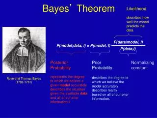
1. P(data|model, I) P(model|data, I) = P(model, I) P(data,I) Likelihood describes how well the model predicts the data Bayes’ Theorem Posterior Probability represents the degree to which we believe a given model accurately describes the situation given the available data and all of our prior information I Prior Probability describes the degree to which we believe the model accurately describes reality based on all of our prior information. Normalizing constant Reverend Thomas Bayes (1702-1761)

2. ml mapping From: Olga Zhaxybayeva and J Peter Gogarten BMC Genomics 2002, 3:4 

3. ml mapping Figure 5. Likelihood-mapping analysis for two biological data sets. (Upper) The distribution patterns. (Lower) The occupancies (in percent)for the seven areas of attraction. (A) Cytochrome-b data fromref. 14. (B) Ribosomal DNA of major arthropod groups (15). From: Korbinian Strimmer and Arndt von HaeselerProc. Natl. Acad. Sci. USAVol. 94, pp. 6815-6819, June 1997

4. (a,b)-(c,d) /\ / \ / \ / 1 \ / \ / \ / \ / \ / \/ \ / 3 : 2 \ / : \ /__________________\ (a,d)-(b,c) (a,c)-(b,d)Number of quartets in region 1: 68 (= 24.3%)Number of quartets in region 2: 21 (= 7.5%)Number of quartets in region 3: 191 (= 68.2%)Occupancies of the seven areas 1, 2, 3, 4, 5, 6, 7: (a,b)-(c,d) /\ / \ / 1 \ / \ / \ / /\ \ / 6 / \ 4 \ / / 7 \ \ / \ /______\ / \ / 3 : 5 : 2 \ /__________________\ (a,d)-(b,c) (a,c)-(b,d)Number of quartets in region 1: 53 (= 18.9%) Number of quartets in region 2: 15 (= 5.4%) Number of quartets in region 3: 173 (= 61.8%) Number of quartets in region 4: 3 (= 1.1%) Number of quartets in region 5: 0 (= 0.0%) Number of quartets in region 6: 26 (= 9.3%) Number of quartets in region 7: 10 (= 3.6%) Cluster a: 14 sequencesoutgroup (prokaryotes) Cluster b: 20 sequencesother Eukaryotes Cluster c: 1 sequencesPlasmodium Cluster d: 1 sequences Giardia

5. Li pi= L1+L2+L3 Ni pi Ntotal Alternative Approaches to Estimate Posterior Probabilities Bayesian Posterior Probability Mapping with MrBayes(Huelsenbeck and Ronquist, 2001) Problem: Strimmer’s formula only considers 3 trees (those that maximize the likelihood for the three topologies) Solution: Exploration of the tree space by sampling trees using a biased random walk (Implemented in MrBayes program) Trees with higher likelihoods will be sampled more often ,where Ni - number of sampled trees of topology i, i=1,2,3 Ntotal – total number of sampled trees (has to be large)

6. Illustration of a biased random walk Figure generated using MCRobot program (Paul Lewis, 2001)

7. COMPARISON OF DIFFERENT SUPPORT MEASURES A: mapping of posterior probabilities according to Strimmer and von Haeseler B: mapping of bootstrap support values C: mapping of bootstrap support for embedded quartets from extended datasets (see fig. 2) Zhaxybayeva and Gogarten, BMC Genomics 2003 4: 37

8. Boostrap Support Values for Embedded Quartets vs. Bipartitions: Performance evaluation using sequence simulations and phylogenetic reconstructions

9. C C C D D D 0.01 0.01 N=8(4) N=4(0) N=5(1) 0.01 A 0.01 0.01 B B A B B A C C D C D D A A B A B B N=13(9) N=23(19) N=53(49)

10. Methodology : Input tree Aligned Simulated AA Sequences (200,500 and 1000 AA) Seq-Gen WAG, Cat=4 Alpha=1 Seqboot 100 Bootstraps ML Tree Calculation FastTree, WAG, Cat=4 Repeat 100 times Extract Highest Bootstrap support separating AB><CD Consense Extract Bipartitions For each individual trees Count How many trees embedded quartet AB><CD is supported

11. Results : Maximum Bootstrap Support value for Bipartition separating (AB) and (CD) Maximum Bootstrap Support value for embedded Quartet (AB),(CD)

12. PAML (codeml) the basic model

13. Vincent Daubin and Howard Ochman: Bacterial Genomes as New Gene Homes: The Genealogy of ORFans in E. coli. Genome Research 14:1036-1042, 2004 The ratio of non-synonymous to synonymous substitutions for genes found only in the E.coli - Salmonella clade is lower than 1, but larger than for more widely distributed genes. Fig. 3 from Vincent Daubin and Howard Ochman, Genome Research 14:1036-1042, 2004

14. Trunk-of-my-car analogy: Hardly anything in there is the is the result of providing a selective advantage. Some items are removed quickly (purifying selection), some are useful under some conditions, but most things do not alter the fitness. Could some of the inferred purifying selection be due to the acquisition of novel detrimental characteristics (e.g., protein toxicity, HOPELESS MONSTERS)?

15. sites model in MrBayes The MrBayes block in a nexus file might look something like this: begin mrbayes; set autoclose=yes; lset nst=2 rates=gamma nucmodel=codon omegavar=Ny98; mcmcp samplefreq=500 printfreq=500; mcmc ngen=500000; sump burnin=50; sumt burnin=50; end;

16. the same after rescaling the y-axis plot LogL to determine which samples to ignore

17. copy paste formula plot row enter formula for each codon calculate the the average probability

18. PAML – codeml – branch model dS -tree dN -tree

19. hy-phy Results of an anaylsis using the SLAC approach

21. Hy-Phy -Hypothesis Testing using Phylogenies. Using Batchfiles or GUI Information at http://www.hyphy.org/ Selected analyses also can be performed online at http://www.datamonkey.org/

22. Example testing for dN/dS in two partitions of the data --John’s dataset Set up two partitions, define model for each, optimize likelihood

23. Example testing for dN/dS in two partitions of the data --John’s dataset Alternatively, especially if the the two models are not nested, one can set up two different windows with the same dataset: Model 1 Model 2

24. Example testing for dN/dS in two partitions of the data --John’s dataset Simulation under model 2, evaluation under model 1, calculate LR Compare real LR to distribution from simulated LR values. The result might look something like this or this