Download
1 / 27
270 likes | 453 Views
Statistical Downscaling of the NCEP CFS Retrospective forecasts (precipitation) over the SE US. Young-Kwon Lim, D.W. Shin, S. Cocke, T. E. LaRow, J. J. O’Brien, and E. P. Chassignet Center for Ocean-Atmospheric Prediction Studies, Florida State University, Tallahassee, FL, USA.

E N D
Statistical Downscaling of the NCEP CFS Retrospective forecasts (precipitation) over the SE US Young-Kwon Lim, D.W. Shin, S. Cocke, T. E. LaRow, J. J. O’Brien, and E. P. Chassignet Center for Ocean-Atmospheric Prediction Studies, Florida State University, Tallahassee, FL, USA
Background and Motivation • Global NCEP/CFS : 1) Retrospective forecasts longer than 20 year period (1981-2006), 2) Widely used in many studies, 3) the low seasonal predictive skill (e.g., precipitation for growing season) in certain areas. • Question: Can we successfully downscale the CFS data which have 2.5 degree resolution and the low skill over several regions?
Why downscaling over the SE USA? • Extremely high temperature and heavy rainfallwith severe storms during summer, resulting in potentialproperty damage and injuries. • The largest areas ofagricultural farmsin the nation. • An accurateforecast with higher spatial resolution is essentialto adapt management, increase profits, reduce production risks, and mitigate damages.
Regional climate simulation in FSU/COAPS • FSU/COAPS Global Spectral Model(FSU/COAPS GSM) has been downscaled to the20km gridresolution byFSU/COAPS nested regional spectral model(FSU/COAPS NRSM) over the southeast US. Dynamical Downscaling • Statistical downscaling model has been also developed. (CSEOF, multiple regression, and stochastic PC generation are used.)
Observation NCEP CFS 0.2° 0.2° (~20km res.) 2.5° 2.5° (~250km res.) CSEOF analysis Training & Predictor : model output Regression Predictand : observation Regressed eigenfunctions of CFS runs used CSEOF PC generation (for the prediction period) Prediction period Eigenfunctions of the Obs. over training period and the Generated PC used Downscaled data construction Withholding different year for Cross-validation Output
Data (Obs. & CFS) and period • Variables : Daily precipitation • Period : 1987 ~ 2005 (Spring (MAM) ~ Summer (JJA) each year (daily)) • Observed data source : National Weather Service Cooperative Observing Program surface data over the southeast US : ~20km×20km • Large-scale data to be downscaled : NCEP/CFS retrospecitve forecasts : 2.5°×2.5°, 10 members with lagged initial conditions. Seasonal integrations starting from February each year.
Results • 2-d seasonalmean field (CFS, Downscaled data, and Observation) • Time series over ~20 years (Interannual variation)for three states (Tallahassee, Jacksonville, Orlando, Miami, Atlanta, Tifton, Birmingham, and Montgomery) • Error variance and correlations • Categorical Predictabilityfor above/below seasonal climatology • Extremes: Frequency of heavy rainfall events per season • Extremes: Frequency of dry spells per season • Application of downscaled data: agricultural model • Realtime forecast (2008 winter)
Overestimation (largest: Georgia) Biased NCEP/CFS fields (comparison with Obs.) Problems? CFS • East > West • Florida is not the wettest region in summer. Obs. MAM JJA
Little change in rainfall amount Seasonal mean field (before and since 2000) NCEP/CFS Downscaling • Similar regional distribution • Rainfall increase • Reduction in bias Observation
Interannual variation at coarse scale (all area averaged seasonal anomaly) • Observed variation is better captured by downscaling. • Several poor captures are found (e.g., before 1990, and 94~97). • CFS overestimates the observed variation. • Anomaly time series : CFS data show smaller amplitude variation. Black : Observation Red : Downscaling Blue : CFS
Interannual variation at regional scale (seasonal anomaly time series) • Better capture of observed variation since 1999. • Several poor captures in the early period (e.g., before 1990, and 1994). Black : Observation Blue : Downscaling Florida Pan. Northern Georgia NE Florida SouthernGeorgia NorthernAlabama Central Florida SouthernAlabama SouthernFlorida
Error variance and Seasonal Anomaly Correlation Corr. (0.3~0.4) • Localized seasonal forecast with a slight increase in Corr. • Reduction in Relative error variance (REV) (≈ 2 0.6~1.4) REV > 2.0 REV < 1 Corr. (0.4~0.6) REV Corr.
Categorical predictability (HSS) for Seasonal anomaly 0.1~0.2 Downscaling CFS 0.0~0.1 • Downscaling: Positive on most grid points (0~0.5) • Skill in overall: Downscaling > CFS and Rescaling (OA) 0.2~0.45 Rescaling (OA) from the CFS with bias-correction
Extremes (Frequency of daily heavy rainfall events) • Observed variation is captured reasonably by downscaling. • Several poor captures are found in early period (before 1995). • Rescaling overestimates the observed variation. Threshold : exceeds 1 std. + climatology Black : Observation Red : Downscaling Blue : Rescaling from the CFS
Categorical predictability (HSS) for the frequency of rainfall extremes 1 std. + climatology Downscaling Rescaling (OA) from the CFS -0.2 ~ 0.1 • Downscaling: Florida and S. Georgia : > 0.1, Alabama and C. Georgia : -0.1 ~ 0.2, • Rescaling: -0.2 ~ 0.2 0.1~0.5 Difference (Down. - Rescaling) ≥0.1
Extremes (Frequency of Subseasonal dry spells) Threshold : a week average < 0.1mm/day • Downscaled data are closer to the observation. • Rescaled data have serious underestimation problem with little amplitude fluctuation. Black : Observation Red : Downscaling Blue : Rescaling from the CFS
Categorical predictability (HSS) for the frequency of dry spells HSS (Downscaling) Threshold : a week < 0.1mm/day • Downscaling: Better prediction in Georgia and Alabama than Florida : -0.1 ~ 0.4, • Rescaling: no skill in terms of HSS. 0.0~0.4
Application example: Downscaled atmospheric data to the crop model Tifton (GA) Crop Yields and Precipitation Red (CFS) Black (Observed) Green (Bias-corrected downscaled CFS) Maize Yields Precipitation
Application example: Realtime seasonal forecasts (2008 winter) CFS Downscaling
Concluding remarks • Precipitation for growing season from NCEP/CFS (~2.5° res.) run have beendownscaled to local scale of ~20km for the SE US. • Downscaling simulates the regional-scale seasonal precipitation with reduction in wet biases. • Correlation, categorical predictability for seasonal anomaly has been improved from the coarsely resolved NCEP/CFS. • Heavy rainfall events: In overall, downscaling better produces the interannual frequency variation than bias-corrected rescaling. • Subseasonal dry spells: Rescaled data show significant underestimation with much smaller amplitude variation than observation. • Application to crop model and realtime forecast.
Statistical downscaling procedure (1) 1. Cyclostationary EOF analysis for the model output and the observation : CSEOF (Kim and North 1997) : analysis technique for extracting the spatio-temporal evolution of physical modes (e.g., seasonal cycle, ENSO, ISOs, etc.) and their long-term amplitude variations. P(r,t)=∑nSn(t) Bn(r,t) Bn(r,t) : time-dependent eigenfunctions, Sn(t) : PC time series. In this study, CSEOF is conducted on both observation and FSUGSM runs over the training period.
Statistical downscaling procedure (2) 2. Multiple regression between the model output and the observation : CSFOF PC time series of the first significant modes of a predictor variable (FSUGSM data) are regressed onto a certain PC time series of the target variable (observation) in the training period. PCTn(t)=∑iαni·PCPi(t)+ε(t) i=1,2,…10 PCTn(t): target PC time series, αni: regression coefficient PCPi(t): predictor PC time series Relationship between model output and the observation is extracted from CSEOF and multiple regression.
Result of multiple regression PC time series ? (training period) forecast period Eigenfunction (from Observation) Regressed Eigenfunction (model) Both are physically consistent.
Result of multiple regression Eigenfunction (from Observation) Regressed Eigenfunction (model)
Statistical downscaling procedure (3) 3. Generating CSEOF PC of the model data over the forecast period from the regressed fields in the training : CSFOF PC time series of the model data are generated for the prediction period. Modeled data and the regressed eigenfunctions identified from training are used. PCn(t)=∑gP(g,t)·Bn+(g,t) PCn(t): the nth mode PC time series for the prediction period g : large-scale grid point Bn+(g,t) : regressed CSEOF eigenfunctions P(g,t): global model anomaly over the prediction period
Statistical downscaling procedure (4) 4. Downscaled data construction from the eigenfunctions of the observation and the generated CSEOF PC time series : D(s,t)=∑nPCn(t)·Bno(s,t) PCn(t) : generated PC time series from the previous step Bno(s,t): CSEOF eigenfunctions of the observation (training period) D(s,t) : downscaled output 5. Generating downscaled output for the entire period (9yrs) by cross-validation framework
Extremes (Frequency of Subseasonal dry spells (anomaly)) Threshold : a week average < 0.1mm/day • Observed variation is captured by downscaling to a certain extent. • Several peaks are not captured well (e.g., 1998 in Florida). • Rescaled data with bias-correction oscillates near zero (significant underestimation). Black : Observation Red : Downscaling Blue : Rescaling from the CFS