Download
1 / 46
460 likes | 635 Views
The Impact of Information Technology on the Temporal Optimization of Supply Chain Performance. Ken Dozier & David Chang Western Research Application Center HICSS 2007 Hawaii International Conference on System Sciences May 23, 2006 January 3-6, 2007 Hilton Waikoloa Village Resort

E N D
The Impact of Information Technology on the Temporal Optimization of Supply Chain Performance Ken Dozier & David Chang Western Research Application Center HICSS 2007Hawaii International Conference on System Sciences May 23, 2006 January 3-6, 2007 Hilton Waikoloa Village Resort Waikoloa, Big Island Hawaii
Objectives • Develop a mathematical artifact that allows optimization of supply chain performance and reduces production times though Information Technology Policies • Provide the basis for an interactive simulation artifact that increases understanding of optimization strategies for supply chain performance and reduces production times though Innovative Information Technology Policies
What is Knowledge ? Truth Knowledge Belief Ontology Epistemology Axiology Universal Social Personal No Debate Diverge on debate Converge on debate Cause Effect Cause Source: “Ten Philosophical Mistakes”, Mortimer J. Adler 1985 Source: “Design Research in the Technology of Information Systems: Truth or Dare.”, Purao, S. (2002).
Design Research Awareness Slides 7 -19 Abduction 20-24 Deduction 25-42 Conclusion 43-46 Source:Takeda, H.. "Modeling Design Processes." AI Magazine, Winter: 37-48.
Business Takes on Many Forms Direction Cooperation Efficiency Proficiency Competition Concentration Innovation Source: “The Effective Organization: Forces and Form”, Sloan Management Review, Henry Mintzberg, McGill University 1991
Flow Oscillations in Supply Chains • Observations • Cyclic phenomena in economics; ubiquitous & disruptive • Example: Wild oscillations in supply chain inventories • MIT “beer game” simulation • Supply chain of only 4 companies for beer production, distribution, and sales • Results of Observations and Simulations • Negative Feedback Systems with Delays Oscillate • Phase dependence of oscillations on position in chain • Understanding of Managements Personality Impact • The sharing of Knowledge has value
Temporal Oscillations (Firms) Source: Gus Koehler, University of Southern California Department of Policy and Planning, 2002
System Dynamic Common Modes of Interaction Between Positive and Negative Feedback Source: System Dynamics, John Sterman, 2000
Exponential Growth • How thick do you think a paper folded in-half 42 times would be? • How thick would it be after 100 folds? Source: System Dynamics, John Sterman, 2000
Exponential Growth The Answers • 42 folds = 440,000 Km (the distance from the earth to the moon.) • 100 folds = 850 trillion times the distance from the earth to the sun! Source: System Dynamics, John Sterman, 2000
The Beer Game Steady state at 4 cases per week. Wilensky, U. (1999). NetLogo. http://ccl.northwestern.edu/netlogo. Center for Connected Learning and Computer-Based Modeling. Northwestern University, Evanston, IL Beer Game Demo Densmore, O. June 2004
Connectivity Model Developed by Dr. Nathan B. Forrester of A.T. Kearney, Atlanta, 2000
The Beer Game - Not Sharing The system after only a single change from 4 to 8 case. Wilensky, U. (1999). NetLogo. http://ccl.northwestern.edu/netlogo. Center for Connected Learning and Computer-Based Modeling. Northwestern University, Evanston, IL Beer Game Demo Densmore, O. June 2004
The Beer Game - Sharing Knowledge sharing, Wilensky, U. (1999). NetLogo. http://ccl.northwestern.edu/netlogo. Center for Connected Learning and Computer-Based Modeling. Northwestern University, Evanston, IL Beer Game Demo Densmore, O. June 2004
Government Dynamics Source: Gus Koehler, University of Southern California Department of Policy and Planning, 2002
Supply Chain Dynamics Source: Gus Koehler, University of Southern California Department of Policy and Planning, 2002
Complex System Dynamics Source: Gus Koehler, University of Southern California Department of Policy and Planning, 2002
Statistical Physics • Proven formalism for “seeing the forest past the trees” • Well established in physical and chemical sciences • Our recent verification with data in economic realm • Simple procedure for focusing on macro-parameters • Most likely distributions obtained by maximizing the number of micro-states corresponding to a measurable macro-state • Straightforward extension from original focus on energy to economic quantities • Unit cost of production • Productivity • R&D costs • Self-consistency check provided by distribution functions
Plasma Theories • Advanced plasma theories are extremely important when one tries to explain, for example, the various waves and instabilities found in the plasma environment. Since plasma consist of a very large number of interacting particles, in order to provide a macroscopic description of plasma phenomena it is appropriate to adopt a statistical approach. This leads to a great reduction in the amount of information to be handled. In the kinetic theory it is necessary to know only the distribution function for the system of particles. Source: University of Oulu, FInland
Market Redefinition Supply-chain Expansion Supply-chain Discovery Business Model Redefinition Business Model Refinement Business Process Redesign Business Process Improvement Stratification Low β High β Seven Organizational Change Propositions Framework, “Framing the Domains of IT Management” Zmud 2002
JITTA • Investigated the β bureaucratic factor and it’s inverse organizational temperature T (dispersion) • Investigate the ability of Stratification to Differentiate impact of IT Investment on output and job creation • Large firms invest in IT to increase output and eliminate jobs • Small firms invest in IT to increase output and expand workforce • Investigate Partition Function Z, Cumulative Distribution Function opened the linkage to Statistical Physics • Dozier-Chang (06) Journal of Information Technology Theory and Application
4000 3500 3000 2500 2000 1500 1000 500 0 0 10 20 30 40 50 60 Maxwell Boltzman Distribution Confirmation Comparison of U.S. economic census cumulative number of companies vs shipments/company (blue diamond points) in LACMSA in 1992 and the statistical physics cumulative distribution curve (square pink points) with β = 0.167 per $106
CITSA 05 • Wave Phenomena in a Supply Chain • Approach: Constrained maximization of microstates corresponding to a macrostate • Opened the Linkage to Fluid Dynamics • Best Paper at Session, 11th International Conference on Cybernetics and Information Technologies, Systems and Applications
Discrete Supply Chain • Start with a simple “Daisy Chain” topology with discrete label N • Nth stage receives information from (N-1) stage and delivers to (N+1) • Simple Static Analysis • Similar to Sound Waves in a Solid N-1 N N+1
Continuous Supply Chain • Replace the discrete variable N by a continuous variable x. • Replace difference equations with differential equations • Draw on Fluid Dynamics and Designate a flow rate through the supply chain with a velocity variable v and a driving force F • v= dx/dt. [1] • F =MA=dv/dt [2]
Partition Function • A quantity that encodes the statistical properties of a system. • It is a function of temperature and other parameters. Many of the statistical physics variables such as free energy can be expressed in terms of the partition function and its derivatives. • Previous statistical physics quasi-static model determined that a distribution of unit costs of production is Maxwell Boltzman (Dozier Chang 05) • Where C(i), unit cost of production • β is the “bureaucratic factor” (inverse of operating temperature T) • Provide Partition Function Z = Σexp[-βC(i)]] [3]
Parametric Force • From the partition function Z we can determine the associated free energy F where Z = exp [-βF] • Statistical Physics formalism provides the framework to assign a force to variations of any parameter ξ • We therefore havef (ξ) = ∂ F/ ∂ξ • We simply assume that F = αf(ξ) [6] • Wheref(ξ) could represent change induced by government incentives • Or f (ξ) could be change induced by a prime contractor’s new requirement
Distribution Function • A differential distribution function f(x,v,t)dxdv denotes the number of production units in the intervals dx and dv at x and v at time t. • ∂f/ ∂t + ∂[fdx/dt]/ ∂x + ∂[fdv/dt]/ ∂v = 0 [7] • A force F that gives the rate at which v changes in time, this equation can be rewritten • ∂f/ ∂t + ∂[fv]/∂x +[∂fF ] / ∂v = 0 [8]
Abduction 3: Vlasov Equation This becomes Vlasov-like equation for f(x,v,t) ∂f/∂t + v∂f/∂x + F ∂f/∂v = 0 [11] This is the equation for collisionless plasmas This is a very useful approximate way to describe the dynamics of a plasma and to consider that the motions of the plasma particles are governed by the applied external fields plus the macroscopic average internal fields, smoothed in space and time, due to presence and motion of all plasma particles.
Basic fluid flow equations Density is # of production units in the interval dx at x and time t • N(x, t) = dvf(x,v,t) [12] • Average flow of the production units V(x,t) = (1/N)vdvf(x,v,t) [13] • Density and velocity conservation equations • ∂N/∂t + ∂[NV]/∂x = 0 [14] • ∂V/∂t +V ∂V/∂x = F1 - ∂P/∂x [15] • F1 is total force per unit dx F 1 = dV/dt • and P is pressure defined by dispersion of velocities • where the dispersion in flow velocities is given by • P= dv(v-V)2 f(x,v,t)/N(x,t) • Velocity dispersion is independent of x and t • ∂V/∂t +V ∂V/∂x = F 1 - (Dv)2∂N/∂x [19] • This implies that the change in velocity flow is impacted by the primary forcing function and the interacting gradients
Supply Chain Normal Modes • Normal Modes are naturally occurring oscillation of a system • If an external force has the same spatial and temporal form as a Normal Mode, amplification can occur • Normal modes are usually obtained by examining the perturbations about the steady state
Normal Mode Expansions • Density Variations • N(x,t) = N0 + N1(x,t) [20] • Velocity Variations • V(x,t) = V0 + V1(x,t) [21] • Substituting [20] and [21] into • ∂N/∂t + ∂[NV]/∂x = 0 [14] • ∂V/∂t +V ∂V/∂x = F 1 - (Dv)2 ∂N/∂x [19] • ∂N1/∂t + V0∂N1/∂x + N0∂V1/∂x = 0 [22] • ∂V1/∂t +V0∂V1/∂x = F 1(x,t) – (∆v)2 ∂N1/∂x [23]
First Order Oscillations • N1(x,t) = N1(x) exp(iωt) [24] • V1(x,t) = V1(x) exp(iωt) [25] • Given • ∂N1/∂t + V0∂N1/∂x + N0∂V1/∂x = 0 [22] • ∂V1/∂t +V0∂V1/∂x = F 1(x,t) – (∆v)2 ∂N1/∂x [23] • Since coefficients are independent of x, the normal mode equations can be expressed in terms of wave number • N1(x) = N1 exp(ikx) [26] • V1(x) = V1(x) exp(ikx) [27]
Propagating Waves • N1(x,t) = N1 exp[i(ωt-kx)] [28] • V1(x,t) = V1 exp[i(ωt-kx)] [29] • Using these forms • ∂N1/∂t + V0∂N1/∂x + N0∂V1/∂x = 0 [22] • ∂V1/∂t +V0∂V1/∂x = F 1(x,t) – (∆v)2 ∂N1/∂x [23] • Becomes • i(ω-kV0)N1 +N0ikV1 = 0 [30] • iN0 (ω-kV0)V1 =- ik(∆v)2N1 [31]
Two Solutions • In order to have none zero values of N1 and V1 • (ω-kV0)2 = k2(∆v)2 [32] • Equation [32] has two solutions • ω+ =k (V0 +∆v) [33] • A propagating supply chain wave that has a velocity equal to the sum of the steady state velocity V0 plus the dispersion velocity ∆v • ω- = k (V0 -∆v) [34] • A propagating supply chain wave that has a velocity equal to the difference of the steady state velocity V0 minus the dispersion velocity ∆v • Dozier, Chang previous work limited either V0 or ∆v to be zero
Interactions • It has been demonstrated that a force F 1(x,t) can be used to accelerate the rate of production in a supply chain • The force will be most effective when it has a component that coincides with the normal mode of the supply chain • This minimizes non destructive interaction • This resonance effect is best seen when using the Fourier decomposition of the Force F
Fourier • F 1(x,t) = (1/2π)∫∫dωdkF1(ω,k)exp[i(ωt-kx)] [35] • Where F1(ω,k) = (1/2π)∫∫dxdtF 1(x,t)exp[-i(ωt-kx)] [36] • Now each component has the form of a propagating wave. These waves are the most appropriate quantities to interact with the normal modes of the supply chain • We go to a higher order of V(x,t) • V(x,t) = V0 + V1(x,t) + V2(x,t) [37] • Substituting into [19] ∂V/∂t +V ∂V/∂x = F 1 - (Dv)2 ∂N/∂x solving for V2(x,t) • N0(∂V2/ ∂t + V0∂V2/∂x) + N1(∂V1/ ∂t +V0∂V1/∂x) + N0 V1∂V1/∂x • = -(∆v)2∂N2/∂x [38]
Convolution • Using convolution for the product terms • ∫∫dxdtexp[-i(ωt-kx)] f(x,t)g(x,t) = • ∫∫dΩdΚf(-Ω+ω,Κ+κ)g(Ω,Κ) [39] • Where • f(Ω,Κ) = ∫∫dxdt exp[(-i(Ωt-Κx)]f(x,t) [40] • g(Ω,Κ) = ∫∫dxdt exp[(-i(Ωt-Κx)]g(x,t) [41] • Interest in net change in V2 changes thatdon’t average 0, V2 (w=0,k=0) requires we know N1 and V1
New Normal Modes • i(ω-kV0)N1 +N0ikV1 = 0 [30] • i(ω-kV0)N1(ω,k) + N0 ikV1(ω,k) = 0 [42] • iN0 (ω-kV0)V1 =- ik(∆v)2N1 [31] • iN0 (ω-kV0)V1(ω,k) =- ik(∆v)2N1(ω,k) + F1(ω,k) [43] • Solutions • N1(ω,k) = -ik F1(ω,k)[(ω-kV0)2 – k2 (∆v)2] -1 [44] • V1(ω,k) = -i{F1(ω,k)/ N0}(ω-kV0)[(ω-kV0)2-k2(∆v)2]-1 [45]
Landau Acceleration • Substitution into ω=0,k=0 components of the Fourier transform • N0(∂V2/ ∂t + V0∂V2/∂x) + N1(∂V1/ ∂t +V0∂V1/∂x) + N0 V1∂V1/∂x = -(∆v)2∂N2/∂x [38] becomes • ∂V2(0,0)/∂t=∫∫ddk(ik/N02)(ω-kV0)2[ω-kV0)2 – k2(∆v)2]-2 F1(-ω,k) F1(-ω,k) [46] • This resembles the quasilinear equation that has long been used to describe the evolution of background distribution of electrons that are subjected to Landau acceleration (Drummond and Pines( 1962)
Conclusions HICSS 07 • Supply chain oscillations can be described by a fluid flow model of production units through a supply chain • There is as normal mode resonance for a supply chain • Any net change in the rate of production in the entire supply chain is due to the gradient interaction and the resonance of the Fourier components from external parametric forces and Fourier components of the normal modes of the supply chain • An Information Technology Infrastructure is most effective when it provides a capability to time the interactions in such a manner as to constructively align the component interaction
Findings • A simple “daisy chain” topology for the IT in a supply chain can be extended to allow the analysis of the optimal timing for external interventions using a fluid dynamics model. • Fluid-like equations for a simple system describe naturally occurring waves that propagate at two velocities . • This model does allow examination of the optimal timing for interventions of these propagations and parametric forces. Something not possible in simulation models to date • The most effective paramedic interventions will be those that use information technologies to apply them so as to mimic the naturally occurring normal modes of the system.
Future Work • Create a simulation artifact that allows understanding of the optimization principles necessary to tune the IT architecture to facilitate the alignment of external disturbances and normal mode interactions cooperative production. • Of particular interest is the minimal amount of IT required for positive cooperation • Expansion of both artifacts to study the effect of a Field Effect Φ and its universal properties on the ability to constructively adapt the supply chain in real time.
Contact Information For more information, please Visit the Learning Center http://wesrac.usc.edu kdozier@usc.edu Google wesrac Google Ken Dozier