Constraint Satisfaction pr oblems
640 likes | 951 Views
Constraint Satisfaction pr oblems. Outline. CSP? Backtracking for CSP Local search for CSPs Problem structure and decomposition. Constraint satisfaction problems. What is a CSP? Finite set of variables V 1 , V 2 , …, V n Finite set of constraints C 1 , C 2 , …, C m

Constraint Satisfaction pr oblems
E N D
Presentation Transcript
Outline • CSP? • Backtracking for CSP • Local search for CSPs • Problem structure and decomposition
Constraint satisfaction problems • What is a CSP? • Finite set of variables V1, V2, …, Vn • Finite set of constraints C1, C2, …, Cm • Nonempty domain of possible values for each variable DV1, DV2, … DVn • Each constraint Ci limits the values that variables can take, e.g., V1 ≠ V2 • A state is defined as an assignment of values to some or all variables. • Consistent assignment: assignment does not not violate the constraints.
Constraint satisfaction problems • An assignment is complete when every value is mentioned. • A solution to a CSP is a complete assignment that satisfies all constraints. • Some CSPs require a solution that maximizes an objective function. • Applications: Scheduling the time of observations on the Hubble Space Telescope, Floor planning, Map coloring, Cryptography
CSP example: map coloring • Variables: WA, NT, Q, NSW, V, SA, T • Domains: Di={red,green,blue} • Constraints:adjacent regions must have different colors. • E.g. WA NT • E.g. (WA,NT) {(red,green),(red,blue),(green,red),…}
CSP example: map coloring • Solutions are assignments satisfying all constraints, e.g. {WA=red,NT=green,Q=red,NSW=green,V=red,SA=blue,T=green}
Constraint graph • CSP benefits • Standard representation pattern • Generic goal and successor functions • Generic heuristics (no domain specific expertise). • Constraint graph = nodes are variables, edges show constraints. • Graph can be used to simplify search. • e.g. Tasmania is an independent subproblem.
Varieties of CSPs • Discrete variables • Finite domains; size dO(dn) complete assignments. • E.g. map coloring • Eight Queens • Variables Q1, …Q8 – position of each queen is columns 1,…,8 • Each variable has domain {1,2,3,4,5,6,7,8} • boolean CSPs, include. Boolean satisfiability (NP-complete) • Infinite domains (integers, strings, etc.) • E.g. job scheduling, variables are start/end days for each job • Need a constraint language e.g StartJob1 +5 ≤ StartJob3. • Linear constraints solvable, nonlinear undecidable. • Continuous variables • e.g. start/end times for Hubble Telescope observations. • Linear constraints solvable in poly time by LP methods.
Varieties of constraints • Unary constraints involve a single variable. • e.g. SA green • Binary constraints involve pairs of variables. • e.g. SA WA • Higher-order constraints involve 3 or more variables. • e.g. cryptharithmetic column constraints. • Preference (soft constraints) e.g. Prof X prefers teaching in the morning whereas Prof why Y prefers teaching in the afternoon. Assigning an afternoon slot for Prof X costs 2 points against the overall objective function whereas a morning slot costs 1. • often representable by a cost for each variable assignment constrained optimization problems.
CSP as a standard search problem • A CSP can easily expressed as a standard search problem. • Incremental formulation • Initial State: the empty assignment {}. • Successor function: Assign value to unassigned variable provided that there is not conflict. • Goal test: the current assignment is complete. • Path cost: as constant cost for every step.
CSP as a standard search problem • This is the same for all CSP’s !!! • Solution is found at depth n (if there are n variables). • Hence depth first search can be used. • Path is irrelevant, so complete state representation can also be used. • Branching factor b at the top level is nd. • Any of d values can be assigned to any of n variables • Eg – 7 states, 3 colors = 21 • At the next level, Branching factor b is (n -1)d. • 6 states • b=(n-l)d at depth l, hence n!dn leaves (only dn complete assignments).
Commutativity • CSPs are commutative. • The order of any given set of actions has no effect on the outcome. • Example: choose colors for Australian territories one at a time • [WA=red then NT=green] same as [NT=green then WA=red] • All CSP search algorithms consider a single variable assignment at a time there are dn leaves.
Backtracking search • Cfr. Depth-first search • Chooses values for one variable at a time and backtracks when a variable has no legal values left to assign. • Uninformed algorithm • No good general performance (see table p. 143)
Backtracking search function BACKTRACKING-SEARCH(csp) return a solution or failure return RECURSIVE-BACKTRACKING({} , csp) function RECURSIVE-BACKTRACKING(assignment, csp) return a solution or failure ifassignment is complete then return assignment var SELECT-UNASSIGNED-VARIABLE(VARIABLES[csp],assignment,csp) for each value in ORDER-DOMAIN-VALUES(var, assignment, csp)do ifvalue is consistent with assignment according to CONSTRAINTS[csp] then add {var=value} to assignment result RRECURSIVE-BACTRACKING(assignment, csp) if result failure then return result remove {var=value} from assignment return failure
Improving backtracking efficiency • Previous improvements introduce heuristics • General-purpose methods can give huge gains in speed: • Which variable should be assigned next? • In what order should its values be tried? • Can we detect inevitable failure early? • Can we take advantage of problem structure?
Minimum remaining values var SELECT-UNASSIGNED-VARIABLE(VARIABLES[csp],assignment,csp) • A.k.a. most constrained variable heuristic • Rule: choose variable with the fewest legal moves • picks a variable that is most likely to cause a failure – prunes search tree • Variable X with zero legal values remaining will be selected. avoids pointless searches through other variables which will always fail when X is finally selected • Which variable shall we try first?
Degree heuristic • Use degree heuristic • Rule: select variable that is involved in the largest number of constraints on other unassigned variables. • Degree heuristic is very useful as a tie breaker. • In what order should its values be tried?
Least constraining value • Least constraining value heuristic • Rule: given a variable choose the least constraining value i.e. the one that leaves the maximum flexibility for subsequent variable assignments.
Forward checking • Can we detect inevitable failure early? • And avoid it later? • Forward checking idea: keep track of remaining legal values for unassigned variables. • Terminate search when any variable has no legal values.
Forward checking • Assign {WA=red} • Effects on other variables connected by constraints with WA • NT can no longer be red • SA can no longer be red
Forward checking • Assign {Q=green} • Effects on other variables connected by constraints with WA • NT can no longer be green • NSW can no longer be green • SA can no longer be green • MRV heuristic will automatically select NT and SA next, why?
Forward checking • If V is assigned blue • Effects on other variables connected by constraints with WA • SA is empty • NSW can no longer be blue • FC has detected that partial assignment is inconsistent with the constraints and backtracking can occur.
Example: 4-Queens Problem X1 {1,2,3,4} X2 {1,2,3,4} 1 2 3 4 1 2 3 4 X3 {1,2,3,4} X4 {1,2,3,4} [4-Queens slides copied from B.J. Dorr CMSC 421 course on AI]
Example: 4-Queens Problem X1 {1,2,3,4} X2 {1,2,3,4} 1 2 3 4 1 2 3 4 X3 {1,2,3,4} X4 {1,2,3,4}
Example: 4-Queens Problem X1 {1,2,3,4} X2 { , ,3,4} 1 2 3 4 1 2 3 4 X3 { ,2,,4} X4 { ,2,3, }
Example: 4-Queens Problem X1 {1,2,3,4} X2 { ,,3,4} 1 2 3 4 1 2 3 4 X3 {,2,,4} X4 {,2,3,}
Example: 4-Queens Problem X1 {1,2,3,4} X2 { ,,3,4} 1 2 3 4 1 2 3 4 X3 { ,,,} X4 { ,2,3, }
Example: 4-Queens Problem X1 { ,2,3,4} X2 {1,2,3,4} 1 2 3 4 1 2 3 4 X3 {1,2,3,4} X4 {1,2,3,4}
Example: 4-Queens Problem X1 {,2,3,4} X2 {,,,4} 1 2 3 4 1 2 3 4 X3 {1, ,3, } X4 {1, ,3,4}
Example: 4-Queens Problem X1 {,2,3,4} X2 {,,,4} 1 2 3 4 1 2 3 4 X3 {1, ,3, } X4 {1, ,3,4}
Example: 4-Queens Problem X1 {,2,3,4} X2 {,,,4} 1 2 3 4 1 2 3 4 X3 {1, , , } X4 {1, ,3, }
Example: 4-Queens Problem X1 {,2,3,4} X2 {,,,4} 1 2 3 4 1 2 3 4 X3 {1, , , } X4 {1, ,3, }
Example: 4-Queens Problem X1 {,2,3,4} X2 {,,,4} 1 2 3 4 1 2 3 4 X3 {1, , , } X4 { , ,3, }
Example: 4-Queens Problem X1 {,2,3,4} X2 {,,,4} 1 2 3 4 1 2 3 4 X3 {1, , , } X4 { , ,3, }
Constraint propagation • Solving CSPs with combination of heuristics plus forward checking is more efficient than either approach alone. • FC checking propagates information from assigned to unassigned variables but does not provide detection for all failures. • NT and SA cannot be blue! • Constraint propagation repeatedly enforces constraints locally
Arc consistency • X Y is consistent iff for every value x of X there is some allowed y • SA NSW is consistent iff SA=blue and NSW=red
Arc consistency • X Y is consistent iff for every value x of X there is some allowed y • NSW SA is consistent iff NSW=red and SA=blue NSW=blue and SA=??? Arc can be made consistent by removing blue from NSW
Arc consistency • Arc can be made consistent by removing blue from NSW • RECHECK neighbours !! • Remove red from V
Arc consistency • Arc can be made consistent by removing blue from NSW • RECHECK neighbours !! • Remove red from V • Arc consistency detects failure earlier than FC • Can be run as a preprocessor or after each assignment. • Repeated until no inconsistency remains
Arc consistency algorithm function AC-3(csp) return the CSP, possibly with reduced domains inputs: csp, a binary csp with variables {X1, X2, …, Xn} local variables: queue, a queue of arcs initially the arcs in csp while queue is not empty do (Xi, Xj) REMOVE-FIRST(queue) if REMOVE-INCONSISTENT-VALUES(Xi, Xj)then for each Xkin NEIGHBORS[Xi] do add (Xi, Xj) to queue function REMOVE-INCONSISTENT-VALUES(Xi, Xj) returntrue iff we remove a value removed false for eachxin DOMAIN[Xi] do if no value y inDOMAIN[Xi]allows (x,y) to satisfy the constraints between Xi and Xj then delete x from DOMAIN[Xi]; removed true return removed
K-consistency • Arc consistency does not detect all inconsistencies: • Partial assignment {WA=red, NSW=red} is inconsistent. • Stronger forms of propagation can be defined using the notion of k-consistency. • A CSP is k-consistent if for any set of k-1 variables and for any consistent assignment to those variables, a consistent value can always be assigned to any kth variable. • E.g. 1-consistency or node-consistency • E.g. 2-consistency or arc-consistency • E.g. 3-consistency or path-consistency
K-consistency • A graph is strongly k-consistent if • It is k-consistent and • Is also (k-1) consistent, (k-2) consistent, … all the way down to 1-consistent. • This is ideal since a solution can be found in time O(nd) instead of O(n2d3) • YET no free lunch: any algorithm for establishing n-consistency must take time exponential in n, in the worst case.
Further improvements • Checking special constraints – use special purpose algorithms rather than general purpose methods • Checking Alldif(…) constraint • E.g. {WA=red, NSW=red} • Checking Atmost(…) constraint
Further improvements • Algorithm • Remove any variable in the constraint that has a singleton domain • delete that variable’s value from the domains of the remaining variables • Repeat • if empty domain is produced or that there are more variables than domain values left – inconsistency detected • Partial assignment {WA = red, NSW = red} • Applying arc inconsistency of the domain of each variable is reduced to {green, blue} • three variables and only two colors – constraint is violated
Further improvements • Resource constraint – Atmost constraint • P1,P2,P3,P4 – groups of people assigned to each of four tasks • constraint –no more than ten personnel are assigned in total • 3,4,5,6 – violates constraint • Flights 271 and 272 – capacity 165 and 385 • Flight271 [0..165] Flight272 [0..385] • Additional constraint – at least 420 people must be carried in total • Flight271 + Flight272 [420]for • Propagating bounds constraints we get • Flight271 [35..165] Flight272 [255..385]