Linear Discriminant Functions Chapter 5 (Duda et al.)

1. Linear Discriminant FunctionsChapter 5 (Duda et al.) CS479/679 Pattern RecognitionDr. George Bebis

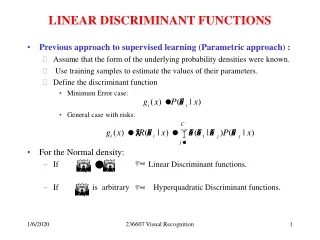
2. Generative vs Discriminant Approach • Generative approaches estimate the discriminant function by first estimating the probability distribution of the patterns belonging to each class. • Discriminant approaches estimate the discriminant function explicitly, without assuming a probability distribution.

3. Generative Approach(case of two categories) • More common to use a single discriminant function (dichotomizer) instead of two: Example: If g(x)=0, then x lies on the decision boundary and can be assigned to either class.

4. Linear Discriminants(case of two categories) • The first step in the discriminative approach is to specify the form of the discriminant. • A linear discriminant has the following form: Decide w1 if g(x) > 0 and w2 if g(x) < 0 If g(x)=0, then x lies on the decision boundary and can be assigned to either class.

5. Linear Discriminants (cont’d)(case of two categories) • The decision boundary g(x)=0 is a hyperplane. • The orientation of the hyperplane is determined by w and its location by w0. • w is the normal to the hyperplane • If w0=0, it passes through the origin • Estimate wandw0using a set of training examples xk.

6. Linear Discriminants (cont’d)(case of two categories) • The solution can be found by minimizing an error function (e.g., “training error” or “empirical risk”): • Use “learning” algorithms to find the solution. true class label: true predicted predicted class label:

7. Geometric Interpretation of g(x) • g(x) provides an algebraic measure of the distance of x from the hyperplane. x can be expressed as follows: direction ofr Substitute x in

8. Geometric Interpretation of g(x) (cont’d) • Substitute x in g(x): since and

9. Geometric Interpretation of g(x) (cont’d) • The distance of x from the hyperplane is given by: setting x=0:

10. Linear Discriminant Functions: multi-category case • There are several ways to devise multi-category classifiers using linear discriminant functions: (1) One against the rest problem: ambiguous regions

11. Linear Discriminant Functions: multi-category case (cont’d) (2) One against another (i.e., c(c-1)/2 pairs of classes) problem: ambiguous regions

12. Linear Discriminant Functions: multi-category case (cont’d) • To avoid the problem of ambiguous regions: • Define c linear discriminant functions • Assign x to wi if gi(x) > gj(x) for all j  i. • The resulting classifier is called a linear machine (see Chapter 2)

13. Linear Discriminant Functions: multi-category case (cont’d) • A linear machine divides the feature space in c convex decisions regions. • If x is in region Ri, the gi(x) is the largest. Note: although there are c(c-1)/2 pairs of regions, there typically less decision boundaries

14. Geometric Interpretation: multi-category case • The decision boundary between adjacent regions Ri and Rj is a portion of the hyperplane Hij given by: • (wi-wj) is normal to Hij and the signed distance from x to Hij is

15. Higher Order Discriminant Functions • Higher order discriminants yield more complex decision boundaries than linear discriminant functions.

16. Linear Discriminants – Alternative Definition • Augmented feature/parameter space: d+1 features d+1 parameters

17. Linear Discriminants – Alternative Definition (cont’d) Classification rule: If αtyi>0 assign yi to ω1 else if αtyi<0 assign yi to ω2 Separates points in (d+1)-space by a hyperplane which passes through the origin. Discriminant:

18. Generalized Discriminants • A generalized discriminant can obtained by first mapping the data to a space of higher dimensionality. • This is done by transforming the data through properly chosen functions yi(x), i=1,2,…, (called φ functions): d  where >> d φ

19. Generalized Discriminants (cont’d) • A generalized discriminant is defined as a linear discriminant in the - dimensional space: φ

20. Generalized Discriminants (cont’d) • Why are generalized discriminants attractive? • By properly choosing the φ functions, a problem which is not linearly-separable in the d-dimensional space, might become linearly separable in the dimensional space!

21. Example d=1 • The corresponding decision regions R1,R2in the 1D-space are not simply connected (not linearly separable). • Consider the following mapping and parameters : Discriminant: or

22. Example (cont’d) • g(x) maps a line in d-space to a parabola in - space. • The problem has now become linearly separable! • The plane divides the -space in two decision regions

23. Learning: linearly separable case(two categories) • Given a linear discriminant function the goal is to “learn” the parameters (weights) α from a set of n labeled samples yi, where each yihas a class labelω1 or ω2.

24. Learning: effect of training examples • Every training sample yi places a constraint on the weight vector α • Visualize solution in “feature space”: • αty=0 defines a hyperplane in the feature space with α being the normal vector. • Given n examples, the solution α must lie within a certain region.

25. Learning: effect of training examples (cont’d) • Visualize solution in “parameter space”: • αty=0 defines a hyperplane in the parameter space with y being the normal vector. • Given n examples, the solution α must lie on the intersection of n half-spaces. parameter space (ɑ1, ɑ2) a2 a1

26. Uniqueness of Solution • Solution vector αis usually not unique; we can impose certain constraints to enforce uniqueness, e.g.,: “Find unit-length weight vector α that maximizes the minimum distance from the training examples to the separating plane”

27. “Learning” Using Iterative Optimization • Minimize an error function J(α) (e.g., classification error) with respect to α: • Minimizeiteratively: α(k) search direction learning rate (search step) α(k+1) How should we choose pk?

28. Choosing pk using Gradient Descent

29. Gradient Descent (cont’d) search space J(α)

30. Gradient Descent (cont’d) • What is the effect of the learning rate h(k) ? η η J(α) slow but converges to solution fast but overshoots solution

31. Gradient Descent (cont’d) • How can we choose the learning rate h(k)? • Need to use Taylor Series expansion Expand f(x) around x0:

32. Gradient Descent (cont’d) • Expand J(a) around a(k) using Taylor Series (up to second derivatives): Hessian (2nd derivatives) Evaluating J(a) at a=a(k+1) and using optimum learning rate Expensive in practice!

33. Choosing pk using Newton’s Method requires inverting H

34. Newton’s method (cont’d) If J(α) is quadratic, Newton’s method converges in one iteration! J(α)

35. Gradient descent vs Newton’s method Gradient Descent Newton

36. “Dual” Classification Problem If αtyi>0 assign yi to ω1 else if αtyi<0 assign yi to ω2 • Ifyi in ω2, replace yi by -yi • Find α such that: αtyi>0 Seek a hyperplane that separates patterns from different categories Seek a hyperplane that puts normalized patterns on the same (positive) side

37. Perceptron rule • The perceptron rule minimizes the following error: where Y(α) is the set of samples misclassified by α. • If Y(α) is empty, Jp(α)=0; otherwise, Jp(α)>0 Find α such that: αtyi>0 for all i

38. Perceptron rule (cont’d) • Apply gradient descent using Jp(α): • Compute the gradient of Jp(α)

39. Perceptron rule (cont’d) missclassified examples

40. Perceptron rule (cont’d) • Keep changing the orientation of the hyperplane until all training samples are on its positive side. a2 Example: a1

41. Perceptron rule (cont’d) η(k)=1 one example at a time Perceptron Convergence Theorem: If training samples are linearly separable, then the perceptron algorithm will terminate at a solution vector in a finite number of steps.

42. Perceptron rule (cont’d) order of examples: y2 y3 y1 y3 “Batch” algorithm leads to a smoother trajectory in solution space.

43. Quiz • Next quiz on “Linear Discriminant Functions” • When: Tuesday, April 23rd