Download

1 / 22
220 likes | 334 Views
This paper discusses an innovative approach to solving elliptic problems using a parallel and domain-decomposed marching method for the Poisson equation. It outlines the basic marching method, introduces a domain decomposition algorithm, and provides a detailed analysis of operation counts associated with this method. The framework addresses error management and the conditions under which the approximations hold true. With a finite difference approach, the study explores the efficiency of the algorithm and presents computational results for a model problem demonstrating the method's effectiveness in large-scale computational domains.

E N D
Parallel and Domain Decomposed Marching Method for Poisson Equation 大氣五 b94209002 簡睦樺
Outline • Basic Marching Method for elliptic problem. • Domain Decomposed Algorithm • Analysis and Operation Counts for this Algorithm • Results
Model Problem • A given open domain of Rn satisfies the following equation for n=1,2,3, f and g are given, and
Finite difference approach With above approach, we can rewrite equation Note that derivative of x and z also use above approach. For i,j,k=0,1,…,N+1, i,j,k=0, N+1 are the boundary condition given.
Approach Idea • If we have the exact solution u and plug into the approach formula, then it should satisfy the equation but there will emerge error with O(δx2). • On the other words, if there exist a data satisfies the plug into the formula, then there must have error at each point.
Testing Result Whether these error comes from a basis? The answer is true.
How to solve these error? • If there exist enough exact data, then the behavior must be control. That is to say, we use the boundary data and have an initial guess next to the boundary points; thus, the error should only exist at the point which comes form the formula marching.
Write down the formula of error u i,j is the exact solution, e is the error.
Error system • We can write the system of error, since they march independently. • Collect each error result at the end of point, we can correct the error by boundary condition of another side. Solve this system, we can get the initial error and correct the marching data by exact solution next to boundary.
Domain Decomposed Algorithm • Although the above method is prefect in idea case, the condition number of the system may easily blow up. • We need another method to solve the problem.
Idea of Domain Decomposed We can find that if we have the marching value at same point, then it must have same value.
Analysis for AlgorithmBasic Algorithm • Data march all domain O(NX*NY*NZ) • Error march all domain O(NX^2*NZ^2*NY) • Compute difference of boundary value O(NX*NZ) • Solve the system O((NX*NZ)^3) • Data march again O(NX*NY*NZ)
An efficient Idea Solve the system, and save the inverse matrix. We need only to take the matrix product when need it. The following is the operation count: 1. Data march all domain O(NX*NY*NZ) 2. Take matrix product O((NX*NZ)^2) 3. Data march again O(NX*NY*NZ) The algorithm has a upper bound O(N^4).
Domain Decomposed Case Unfortunately, domain decomposed case require to solve a larger system than before. Although we prove that the domain decomposed case has a same upper bound compared to usually problem, but the lower bound is rather small than before. i.e.
Analysis • Data march all domain O(NX*NY*NZ) • Error march all domain O(NX^2*NZ^2*NY) • Compute difference of boundary value O(NX*NZ*NY) • Solve the system O((NX*NY*NZ)^3) • Data march again O(NX*NY*NZ) This step is relative to size of sub-domain.
The efficient solver 1. Data march all domain O(NX*NY*NZ) 2. Take matrix product O((NX*NY*NZ)^2) 3. Data march again O(NX*NY*NZ) The algorithm has a upper bound O(N^6). Remark. NY>>NB
Convergent table and log-log plot Least squares fit gives E(h) = 0.003 * h^1.54
24*24*24 Case Least squares fit gives E(h) = 18.0 * h^0.8