Download
1 / 37
370 likes | 529 Views
Tonga Institute of Higher Education Design and Analysis of Algorithms. IT 254 Lecture 5: Advanced Design Techniques. Advanced Design Techniques. Other methods of design, like divide-and-conquer and randomization, can usually be applied to many problems.

E N D
Tonga Institute of Higher EducationDesign and Analysis of Algorithms IT 254 Lecture 5: Advanced Design Techniques
Advanced Design Techniques • Other methods of design, like divide-and-conquer and randomization, can usually be applied to many problems. • There are newer techniques that are a little more complicated, but allow computer scientists to solve harder problems. We will look at two methods. • "Greedy" programming is a way to optimize a solution where you must make a choice. In this method, you make the best choice at each time and by the end you will have made the best choice overall • "Amortized Analysis" is a tool for analyzing algorithms that allows us to look at algorithms where the running time changes depending on input, and then to find the average "amortized" running time.
Greedy Algorithms • Optimization problems is a category of problems that focus on finding the best solution. • In these problems, there can be many possible solutions. Each solution has a value and the goal is to find the solution with the optimal (maybe maximum or minimum) value. • Greedy algorithms are a technique used to solve these problems. • A greedy algorithm will always make the choice that looks best at the moment it makes it. • In mathematical words: It makes the locally optimal choice, hoping that it will lead to the globally optimal choice.
Greedy Algorithm: Activity Selection • The first example we will look at is an activity selector. • Suppose there is a set S = { 1,2, … n } of n proposed activities that all need to use a resource. • For example, a classroom which can only be used by one class at a time. • Each activity "i" has a start time and a finish time so that starti < finishi • The activity selection problem is to select a maximum size set of activities that all can use a resource. • For this problem, we assume that all activities are sorted in order of increasing finish time: • f1 < f2 < f3 < … < fn
Activity Selector • We can use the following pseudo-code to demonstrate a greedy algorithm to solve the problem. • Here "A" is the set of all activities. "j" is the last activity added. Since activities are listed in sorted order, fj is always the maximum finishing time of any activity in A. • So fj = max { fk: k Э A } • Lines 3-4 select the first activity and put it in A • Lines 5-8 add an activity in the start time that is after the finishing time of the last thing added. • This is a O(n) algorithm if activities are sorted before the algorithm 1:Greedy-Selector 2: n = length of Set 3: A = new Array(1) 4: j = 1 5: for i = 2 to n 6: if si > fj 7: A = A υ { i } 8: j = i 9: return A
Activity Selector • The activity picked next by the algorithm is always the one with the earliest finish time that can be scheduled without conflicts. • The activity picked is thus the "greedy" choice, because it does not look at all choices, but only the best one it sees right in front of it. • The greedy choice maximizes the amount of unscheduled time.
Greedy Properties • How do we know if the Greedy Algorithm is the best choice for solving a problem? • The first important thing to know about is if a globally optimal solution can be gotten by making locally optimal solutions. • This means, can we get the best answer for the whole problem, by making good answers for smaller problems. • This means that we can sometimes use induction to help us see if the problem can be solved with a greedy algorithm.
Properties: Optimal Substructure • "Optimal substructure" is an important property for a problem to have if you want to solve it using a greedy method • Optimal substructure means the best solution to a problem is made of the best solutions to sub-problems inside of it • The Activity Selector was an example of this. • The sub problem was: which activity added to the list will maximize the size of the list right now. • After solving each of these sub-problems, we have an answer that solves the whole problem
Greedy Algorithms: Compression • "Huffman coding" is a method to compress data. • The main idea of data compressions is that you start with an original thing x (text, picture, movie) and you want to change x with a function C(x) so that C(x) has fewer bits than x • But you also want a way to change C(x) back into x, with a function D(x) • Thus: D(C(x)) = x • C(x) = compress x • D(x) = decompress x
Compression • There are two types of compression algorithms, • Lossless Compression: D(C(x)) = x • Lossy Compression: D(C(x)) ≈ x • Things that compress text or programs should be lossless, but things like pictures and sound can be lossy • (You don’t want words from a book to be almost the same as words from a book) • (But with a picture, if the quality is not perfect you will not notice that much)
Huffman Compression • Huffman compression can give savings of 20-90% most of the time, depending on the data being compressed. • Huffman's greedy algorithm uses a table of the frequencies of occurrence for each character to build an optimal way of representing a character as a binary string. • This means that it will count how many times it sees each letter and make a table of the counts. Then it will find the shortest binary strings (like "01010") that will map to the letter that occurs the most.
Huffman Compression • Huffman will do compression based on a "variable-length" code. This means that characters that occur more often will use fewer bits, while characters that do not occur often will use more bits. • A "fixed-length" code means every character has the same amount of bits used to save it. • For example, what if we have a book with 100,000 letters that we want to compress
Huffman Compression • In the "fixed-length" coding we need 3 bits for each character and there are 100,000 characters. Thus, 300,000 bits are needed • In the variable length code, we can do better. • (45*1 + 13*3 + 12*3 + 16*3 + 9*4 + 5*4) = 224,000 bits. • This saving is about 25% better than the fixed length
Huffman Compression • If you noticed the variable lengthed codes from before, there was one character that had a 1 bit code, but there was no two bit codes. • This is because Huffman uses "prefix codes." This means that a used code is never the same as the beginning of another code. (Prefix means the part of a word that comes in the beginning) • This makes encoding and decoding much easier if we follow this rule. • For example: abc = 0 + 101 + 100 = 0101100 • And 001011101 = 0 + 0 + 101 + 1101 = aabe • Prefix codes make sure that we always get the same thing out that we put in ( D(C(x)) = x )
Huffman • The decoding needs an easy way to find which letter belongs to a mapping. • A binary tree is a good data structure for this. • The leaves of the tree will be a character and the paths will represent either 0 or 1. • 0 can mean "go to the left child" • 1 can mean "go to the right child" • This also means we can easily know how many bits we need to save the data. • Cost = SumAllCharacters(height(c) * count(c)) where "c" is a character • Or Cost =
Example Trees Fixed Length Codes Variable Length Codes Each node stores the total number of characters in the sub tree below. The leaves contain the character and the number of occurrences. We can see that a variable length code tree may become very unbalanced
Huffman Coding • Huffman invented a greedy algorithm that will find the variable length codes and build the tree in a bottom up manner. • C is a set of n characters. • Q is a Priority Queue that holds and sorts all the characters by frequency • The for loop keeps taking out the two minimum nodes and making them children of z, a new node that holds the total frequency count • Then we insert z back into the Queue until we have done this for each character. • Lastly, we return the Extract-Min which is the root of the tree Huffman(C) n = length of C Q = C for i = 1 to n – 1 z = new Node() z->left = Extract-Min(Q) z->right = Extract-Min(Q) z->count = z->left->count + z->right->count Insert(Q,z) return Extract-Min(Q)
Huffman Tree Building A B C D E F
Huffman Trees • The Huffman coding uses a greedy algorithm because it has an "optimal substructure." • This means that if it is able to solve small problems correctly, then it can put the small problems together to get the best solution for the whole problem • In the Huffman codes, we solve a prefix code problem for two nodes at a time. We "greedily" choose the two smallest nodes and then work on the next two smallest. • This process demonstrates how to use greedy algorithms to solve a problem that would otherwise be difficult
Amortized Analysis • Amortized analysis is the time required to do a sequence of operations averaged over all the operations done. • We have looked at the worst-case running times of individual operations, but… • Sometimes the cost of a single operation changes a lot, so the worst case is not so good. • Instead, we want to look at the average cost of an operation over a series of operations. • This is different from the “Average-case” analysis. • Amortized analysis looks at the average cost of an operation. Average-case looks at how long an entire function will take on average
Amortized • Thus, “amortized time” means: • If any sequence of n operations take < T(n) time, the amortized time per operation is T(n)/n • Also, if the amortized time of one operation is U(n), then any sequence of n operations takes n*U(n) time • This average is over a sequence of operations for any sequence • Not the average for an input distribution • Not the average over random choices made by an algorithm • Amortized analysis: a way to express an algorithm in such a way that even if the worst case is bad, the total performance of a sequence of operations is not always bad
Amortized Analysis • Method One: Accounting method • Charge each operation an amortized cost • Amount not used stored in “bank” • Later operations can used stored credit • Balance must not go negative • Method Two: Aggregate method of amortized analysis: • n operations take time T(n) • Average cost of an operation = T(n)/n
Dynamic Tables • What if we want to make a table, like a hash table, for dynamic data (data that changes). And we want to make it as small as possible • Problem: if too many items inserted, table may be too small for all of them, so… • Solution: get more memory if we need it
Dynamic Tables 1. Initialize table to size m = 1 2. Insert elements until n elements > m 3. Generate new table of size 2m 4. Reinsert old elements into new table 5. (back to step 2) • What is the worst-case cost of an insert? • One insert can be costly, but the total?
Analysis Of Dynamic Tables • Let ci = cost of ith insert • ci = i if i-1 is exact power of 2, • 1 otherwise • Example: • Operation Table Size Cost Insert(1) 1 1 1
Analysis Of Dynamic Tables • Let ci = cost of ith insert • ci = i if i-1 is exact power of 2, • 1 otherwise • Example: • Operation Table Size Cost Insert(1) 1 1 1 Insert(2) 2 1 + 1 2 Insert(3) 4 1 + 2 3
Analysis Of Dynamic Tables • Let ci = cost of ith insert • ci = i if i-1 is exact power of 2, • 1 otherwise • Example: • Operation Table Size Cost Insert(1) 1 1 1 Insert(2) 2 1 + 1 2 Insert(3) 4 1 + 2 3 Insert(4) 4 1 4 Insert(5) 8 1 + 4 5
Analysis Of Dynamic Tables • Let ci = cost of ith insert • ci = i if i-1 is exact power of 2, • 1 otherwise • Example: • Operation Table Size Cost Insert(1) 1 1 1 Insert(2) 2 1 + 1 2 Insert(3) 4 1 + 2 3 Insert(4) 4 1 4 Insert(5) 8 1 + 4 5 Insert(6) 8 1 6 Insert(7) 8 1 7 Insert(8) 8 1 8
Analysis Of Dynamic Tables • Let ci = cost of ith insert • ci = i if i-1 is exact power of 2, • 1 otherwise • Example: • Operation Table Size Cost 1 2 3 4 5 6 7 Insert(1) 1 1 8 1 Insert(2) 2 1 + 1 9 2 Insert(3) 4 1 + 2 Insert(4) 4 1 Insert(5) 8 1 + 4 Insert(6) 8 1 Insert(7) 8 1 Insert(8) 8 1 Insert(9) 16 1 + 8
Aggregate Analysis: Dynamic Tables • "n" Insert() operations cost: • Average cost of operation = (total cost)/(# operations) < 3n/n < 3 • So we can say a dynamic table costs the same as a fixed-size table • Both O(1) per Insert operation, even though in the dynamic table some operations are really bad.
Accounting Analysis • We can also use another form of amortized analysis, called the "accounting method". • For our dynamic table we can "charge" each operation $3 amortized cost • Use $1 to perform immediate Insert() • Store $2 • When table doubles • Use the saved $2 to reinsert two old items • We’ve "paid" these costs with the last n/2 Insert()s • Benefit: O(1) amortized cost per operation
Accounting Analysis • Suppose we also must support insert & delete. • Then the table could shrink and grow • Table overflows double it (as before) • Table < 1/4 full halve it • Charge $3 for Insert (as before) • Charge $2 for Delete • Store extra $1 in emptied slot • Use later to pay to copy remaining items to new table when shrinking table • We only need extra $1 because we're reinserting fewer items
Example: Binary Counter • Consider the following problem: • You want a binary counter that does n Increment operations • We use an array A that holds bits so that • A[i] = 0 or • A[i] = 1 • A[0] is lowest order bit, so value of counter is • X = SUM(A[i]*2i) from i n • Algorithm • Increment(A) • A[0] = A[0]+1 • i = 0 • while (A[i] == 2) • A[i+1] = A[i+1] + 1; • A[i] = 0; • i++
Example: Binary Counter • The running time of Increment is the number of iterations of the while loop • Examples: • X = 47 A = <0,…,0,1,0,1,1,1,1 > • X = 48 A = <0,…,0,1,1,0,0,0,0 > • X = 49 A = <0,…,0,1,1,0,0,0,1 > • Increment from x = 47 to x = 48 has cost 5 • Increment from x = 48 to x = 49 has cost 1
Example: Binary Counter • Analysis of a sequence of n increments • Number of bits in representation of n is log n, thus n operations = O(n) * O(lg n) = O(n lg n) • Amortized running time of Increment is O(1) for one operation, O(n) for n operations • A[0] will flip on every increment (n times) • A[1] will flip on every second increment (n/2 times) • A[2] will flip on every third increment (n/4) • A[i] will flip on every 2i increment (n/2i times) • Total running time T(n) = Σ(n/2i) from i=0 to log n • T(n) = Σ(n/2i) to lg n < Σ (1/2i) to ∞ = 2n = O(n) • Amortized cost for one operation O(2n)/n = O(2)
Example: Binary Counter • Accounting Analysis: • Every 1 in A will hold one credit • Change from 1 -> 0 paid using a credit • Change from 0 -> 1 paid by Increment. Pay one credit to do the flip and place one credit on new 1 • Increment cost O(1) amortized.
Summary • Advanced design techniques should be put in your mind in case you run across a problem that seems especially difficult. • Greedy algorithms can be very helpful in solving problems that would seem hard to program. • Amortized analysis is not really a way to program, but is instead a way to find out running times. • What it does special is that it realizes that different operations and different input may change the running time. • In these cases, we may be more interested in an average running time of an operation, instead of the worst case of an algorithm.