Math.375 III- Interpolation
340 likes | 363 Views
Math.375 III- Interpolation. Vageli Coutsias. Problems. Polynomial Interpolation in 1d: VanderMonde and Newton Piecewise linear and cubic interpolation in 2d Matrices and BW images Color Images. function a = InterpV (x,y) n = length(x); V = ones(n,n); for j = 2:n

Math.375 III- Interpolation
E N D
Presentation Transcript
Math.375 III- Interpolation Vageli Coutsias
Problems • Polynomial Interpolation in 1d: VanderMonde and Newton • Piecewise linear and cubic interpolation in 2d • Matrices and BW images • Color Images
function a = InterpV(x,y) n = length(x); V = ones(n,n); for j = 2:n V(:,j) = x.*V(:,j-1); end a = V\y;
function pVal = HornerV(a,z) n = length(a); m = length(z); pVal = a(n)*ones(size(z)); for k = n-1:-1:1 pVal = z.*pVal + a(k); end
function c = InterpNRecur(x,y) n = length(x); c = zeros(n,1); c(1) = y(1); if n > 1 c(2:n) =InterpNRecur(x(2:n), ((y(2:n)-y(1))./(x(2:n)-x(1))); end
function c = InterpN(x,y) n = length(x); for k = 1:n-1 y(k+1:n) = (y(k+1:n)-y(k))/(x(k+1:n)-x(k)); end c = y;
function pVal = HornerN(c,x,z) n = length(c); pVal = c(n)*ones(size(z)); for k=n-1:-1:1 pVal = (z-x(k)).*pVal + c(k); end
for i = 1:m+1 %Equally Spaced, m=16 x(i,1) = .5*(b+a) +.5*(b-a)*(2*(i-1)-m)/m ; end y = 1./(1+ll*x.^2); [P,S] = polyfit(x,y,16); pVal = polyval(P,x0);
% least squares fit: degre 8 fit based on 17 pts. [P,S] = polyfit(x,y,8); pVal = polyval(P,x0);
for i = 1:m+1 % Chebyshev Nodes x(i,1) = .5*(b+a) +.5*(b-a)*cos(pi*(i-1)/m) ; end y =1./(1+ll*x.^2); a = InterpN(x,y); pVal = HornerN(a,x,x0);
Typical picture with its characteristics [X,map]=imread('Mars','gif'); image(X); colormap(map); class(X) = uint8; size(X) = 1381 512
0 1600 X 0 JPG: RGB format 1200 >[x,y]=ginput(1) >[x,y] 500 353 Size(X): 1200,1600, 3 class(X): uint8 Y
function z = LinInterp2Dc(xc,yc,a,b,c,d,fA) [n,m,r] = size(fA); hx = (b-a)/(n-1); i = max([1 ceil((xc-a)/hx)]); dx = (xc - (a+(i-1)*hx))/hx; hy = (d-c)/(m-1); j = max([1 ceil((yc-c)/hy)]); dy = (yc - (c+(j-1)*hy))/hy; for k=1:r z(k) = uint8((1-dy)*((1-dx)*double(fA(i, j, k)) +dx *double(fA(i+1, j, k))) +dy *((1- dx)*double(fA(i, j+1,k)) +dx *double(fA(i+1,j+1,k)))); end
(i+1,xc) j (i+1,xc) dx (yc,j) (yc,j+1) hy dy (yc,xc) (i,j) hx (i,xc) i Stencil for bilinear interpolation
j=1 j=N-1 X i=1 (i,j) (yc,xc) i=N-1 Y
For an interior grid point, choose symmetric neighbors for interpolation.
j=1 j=N-1 X i=1 (1,j) (yc,xc) i=N-1 Y
For a boundary point, choose one-sided neighbors for interpolation in the bounded direction, and symmetrically in the other.
j (i-1,xc) (i,j) (i,xc) dy hy dx (yc,xc) (i+1,xc) hx (i+2,xc) i Stencil for bicubic interpolation
f(i,j) p3(xc) f(i,xc) j+2 j-1 x(j) j+1 xc for ii=i-1:i+2 [Px,S] = polyfit(x(j-1:j+2),f(ii,j-1:j+2),3); pc(ii,xc) = polyval(Px,xc); end [Py,S] = polyfit(y(i-1:i+2),pc(j-1:j+2,xc),3); pc(yc,xc) = polyval(Py,yc);
%----------Input center and radius of area to magnify clear all close all [X,map]=imread('Mars','gif'); image(X); colormap(map); % circles i1 = zeros(2,2); sprintf 'click center of image' i1(1,:)=ginput(1); sprintf 'click point on circumference of image' i1(2,:)=ginput(1); C(1,:) = [ ceil(i1(1,1)) ceil(i1(1,2))]; RR = ceil(sqrt((i1(2,1)-i1(1,1))^2+((i1(2,2))-i1(1,2))^2)) %---------------------------------------------
%--------------------------------------------- % convert to square centered at Ci n11 = ceil(C(1,1)-RR); n12 = ceil(C(1,1)+RR); m11 = ceil(C(1,2)-RR); m12 = ceil(C(1,2)+RR); mm = m12 - m11+1; nn = n12 - n11+1; B = X(m11:m12, n11:n12); figure %original segment image(B);colormap(map);
% Now magnify contents gradually for k = [2,4,8] Z = zeros(k*mm,k*nn); for i=1:k*mm for j=1:k*nn yc = i/k; xc = j/k; Z3(i,j) = CubicInterp2Dc(yc,xc,1,mm,1,nn,B); Z1(i,j) = LinInterp2Dc(yc,xc,1,mm,1,nn,B); end end figure;image(Z1);colormap(map); figure;image(Z3);colormap(map); end
Original: dust devil on Mars’s South
As prev., linear int. at 4x density
As prev., cubic int. at 4x density
j=1 j=N-1 X i=1 i=N-1 Y Pay attention to corners!
Input-output structures • x=input(‘string’) • title=input(‘Title for plot:’,’string’) • [x,y]=ginput(n) • disp(‘a 3x3 magic square’) • disp(magic(3)) • fprintf(‘%5.2f \n%5.2f\n’,pi^2, exp(1))
Writing to and reading from a file fid = fopen('output','w') a=linspace(1,100,100); fprintf(fid,'%g degC = %g degF\n',a,32+1.8*a); fid=fopen('output','r') x=fscanf(fid,'%g degC = %g degF'); x=reshape(x,(length(x)/2),2)
---------------------------------------- I. A=[1 2 3;4 5 6;7 8 9]; y=x'; %transpose x=zeros(1,n); length(x); x=linspace(a,b,n); a=x(5:-1:2); %SineTable (Help SineTable) disp(sprintf('%2.0f %3.0f ',k, a(k))); ----------------------------------------
-------------------------------------------------------------------------------------------------------------------------------- II. VECTOR OPERATIONS: (1) vector: scale, add, subtract (scalar*vector) 2*[10 20 30] = [20 40 60] (2) POINTWISE vector: multiply, divide, exponentiate (pointwise vector * vector) [2 3 4].*[10 20 30] = [20 60 120] (for pointwise operations, dimensions must be identical!) (3) Setting ranges for axes, Superimposing plots: plot(x,y,x,exp(x),'o') axis([-40 0 0 0.1]) using "hold on/off" extended parameter lists (4) Subplots: subplot(m,n,k) (5) Vector linear combos: matrix*vector (6) Tensor Products (x is array, A is array of arrays of same shape as x) A=[f1(x) f2(x) ... fn(x)] A(k,:) k-th row; A(:,i) i-th column (7) loops: loop until ~condition or for fixed no. of times while any(abs(term) > eps*abs(y)) for term = 1:n end (8) size(A) gives array dimensions (array, can be used to index other arrays) length(x) gives vector dimension ----------------------------------------------------------------
-------------------------------------------------------------------------------------------------------------------------------- II' (Miscellaneous topics) rem(x,n): remainder if x == 1 (< <= == >= > ~=) (& and; | or; ~ not; xor exclusive or) else endif s3 = [s1 s2]; concatenation of strings, treated like arrays [xmax, imax] = max(x); (max val, index) rat = max(x)/x(1) x(1) = input('Enter initial positive integer:') density = sum(x<=x(1))/x(1);
Summary • Interpolation • vanderMonde, Newton, Least Squares • 2d interpolation: linear and cubic • Color figures and uint8 • Smoothing of images
References • find m-files at www.math.unm.edu/~vageli • Higham & Higham, Matlab Handbook • C.F.van Loan, Intro to Sci.Comp. (2-3)