Download
1 / 36
360 likes | 567 Views
From the Universe to Relativistic Heavy-Ion Collisions: CMBR Fluctuations and Flow Anisotropies. Ajit M. Srivastava Institute of Physics Bhubaneswar, India. Outline: Relativistic heavy-ion collision experiments (RHICE): Anisotropies in particle momenta for non-central collisions,

E N D
From the Universe to Relativistic Heavy-Ion Collisions: CMBR Fluctuations and Flow Anisotropies Ajit M. Srivastava Institute of Physics Bhubaneswar, India
Outline: • Relativistic heavy-ion collision experiments (RHICE): • Anisotropies in particle momenta for non-central collisions, • Elliptic Flow and flow fluctuations • 2. Applying CMBR analysis techniques to RHICE. • Deeper correspondence with CMBR anisotropies: Recall – • Inflationary superhorizon density fluctuations, coherence • and acoustic peaks in CMBR anisotropy power spectrum • Argue: These crucial aspects present in RHICE also • (Mishra, Mohapatra, Saumia, AMS) • Concluding Remarks. • Talk of Saumia P.S. in Parallel 3B Session: • Effects of magnetic field: on CMBR acoustic peaks, and in RHICE: Enhancement of flow anisotropies, larger v2 • possibility of accommodating a larger value of η/s ? • (Mohapatra, saumia, AMS)
Relativistic heavy-ion collision experiments (RHICE): QGP phase a transient stage, lasts for ~ 10-22 sec. Finally only hadrons detected carrying information of the system at freezeout stages (chemical/ thermal freezeout). Often mentioned: This is quite like CMBR which carries the information at the surface of last scattering in the universe. Just like for CMBR, one has to deduce information about The earlier stages from this information contained in hadrons Coming from the freezeout surface. We have shown that this apparent correspondence with CMBR is in fact very deep There are strong similarities in the nature of density fluctuations in the two cases (with the obvious difference of the absence of gravity effects for relativistic heavy-ion collision experiments). First note: Flow anisotropies and Elliptic flow
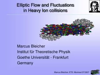
Recall: Elliptic Flow in RHICE In non-central collisions: central QGP region is anisotropic collision along z axis y central pressure = P0 Outside P = 0 Collision region x z Spectators Anisotropic shape implies: Recall: Initially no transverse expansion Anisotropic pressure gradient implies: Buildup of plasma flow larger in x direction than in y direction Spatial eccentricity decreases
y Initial particle momentum distribution isotropic : it develops anisotropy due to larger flow in x direction This momentum anisotropy is characterized by the 2nd Fourier coefficient V2 x (Elliptic flow) Earlier discussions mostly focused on a couple of Fourier Coefficients, with n = 2, 4, 6, 8 (Note: no odd harmonics) Importantly: mostly discussion on average values of (with the identification of the event plane). Few discussions about fluctuations of for n = 2,4
First argued by us: Inhomogeneities of all scales present, even in central collisions: Arising from initial state fluctuations These anisotropies were known earlier, however, they were only discussed in the context of determination of the eccentricity for elliptic flow calculations. We argued that due to these initial state fluctuations: All Fourier coefficients are of interest (say, n=1 to 30 -40, including Odd harmonics). However more important to Calculate root-mean-square values, and NOT the average values.
Contour plot of initial (t = 1 fm) transverse energy density for Au-Au central collision at 200 GeV/A center of mass energy, obtained using HIJING Azimuthal anisotropy of produced partons is manifest in this plot. (Recall: Hirano’s Talk) Thus: reasonable to expect that the equilibrated matter will also have azimuthal anisotropies (as well as radial fluctuations) of similar level
This brings us to our first proposal for correspondence Between CMBR physics and physics of heavy-ion collisions Recall: for the case of the universe, density fluctuations are accessible through the CMBR anisotropies which capture imprints of all the fluctuations present at the decoupling stage: For RHICE: the experimentally accessible data is particle momenta which are finally detected. Initial stage spatial anisotropies are accessible only as long as they leave any imprints on the momentum distributions (as for the elliptic flow) which survives until the freezeout stage. So: Fourier Analyze transverse momentum anisotropy of final particles (say, in a central rapidity bin) in a reference frame with fixed orientation in the lab system for All Events.
The most important lesson for RHICE from CMBR analysis CMBR temperature anisotropies analyzed using Spherical Harmonics Now: Average values of these expansions coefficients are zero due to overall isotropy of the universe However: their standard deviations are non-zero and contain crucial information. This gives the celebrated Power Spectrum of CMBR anisotropies Lesson : Apply same technique for RHICE also
For central events average values of flow coefficients will be zero (same is true even for non-central events if a coordinate frame with fixed orientation in laboratory system is used). Following CMBR analysis, we propose to calculate root-mean-square values of these flow coefficients using a lab fixed coordinate system, And plot it for a large range of values of n = 1, 30-40 These values will be generally non-zero for even very large n and will carry important information Important: No need for the identification of any event plane So: Analysis much simpler. Straightforward Fourier series expansion of particle momenta We will see that such a plot is non-trivial even for large n ~ 30-40
We estimate spatial anisotropies for RHICE using HIJING event generator We calculate initial anisotropies in the fluctuations in the spatial extent R(f) (using initial parton distribution from HIJING) R(f) represents the energy density weighted average of the transverse radial coordinate in the angular bin at azimuthal coordinate f. We calculate the Fourier coefficients Fn of the anisotropies in where R is the average of R(f). Note: We represent fluctuations essentially in terms of fluctuations in the boundary of the initial region. May be fine for estimating flow anisotropies, especially in view of thermalization processes operative within the plasma region
Contour plot of initial (t = 1 fm) transverse energy density for Au-Au collision at 200 GeV/A center of mass energy, obtained using HIJING
We use: Momentum anisotropy v2 ~ 0.2 spatial anisotropy e. For simplicity, we use same proportionality constant for all Fourier coefficients: Just for illustration of the technique Note: we are just modeling the momentum anisotropy using Spatial anisotropies Proper values for momentum anisotropies will come from hydrodynamics simulations Note: (Again, recall from discussion in Hirano’s talk): For small amplitudes of fluctuations, each harmonic will evolve independently. So, proportionality of spatial anisotropy harmonic to momentum anisotropy harmonic for each mode is reasonable.
Important: In contrast to the conventional discussions of the elliptic flow, we do not try to determine any special reaction plane on event-by-event basis. A coordinate system with fixed orientation in the Lab frame is used for calculating azimuthal anisotropies for all the events. Thus: This is why, averages of Fn (and hence of vn) vanishes when large number of events are included in the analysis. However, the root mean square values of Fn , and hence of vn , will be non-zero in general and will contain non-trivial information.
Results: Just like power spectrum for CMBR, non-zero values are obtained from HIJING for all n = 1- 30 HIJING parton distribution Errors less than ~ 2% Uniform distribution of partons Important: Irrespective of its shape, such a plot has important information about the nature of fluctuations (specially initial ones)
For non-central collisions, elliptic flow can be obtained directly From such a plot b = 8 fm b = 5 fm b =0
Recall: Acoustic peaks in CMBR anisotropy power spectrum Solid curve: Prediction from inflation So far we discussed: Plot of for large values of n will give important information about initial density fluctuations. We now discuss: Such a plot may also reveal non-trivial structure like acoustic peaks for CMBR.
We have noted that initial state fluctuations of different length scales are present in Relativistic heavy-ion collisions even for central collisions The process of equilibration will lead to some level of smoothening. However, thermalization happens quickly (for RHIC, within 1 fm) No homogenization can be expected to occur beyond length scales larger than this. This provides a natural concept of causal Horizon Thus, inhomogeneities, especially anisotropies with wavelengths larger than the thermalization time scale should be necessarily present at the thermalization stage when the hydrodynamic description is expected to become applicable. As time increases, the causal horizon (or, more appropriately, the sound horizon) increases with time. Note: we are discussing Causal horizon in transverse direction as relevant for flow anisotropies. Earlier discussions of causal horizon only referred to longitudinal directions.
This brings us to the most important correspondence between the universe and relativistic heavy-ion collisions: It is the presence of fluctuations with superhorizon wavelengths. Recall: In the universe, density fluctuations with wavelengths of superhorizon scale have their origin in the inflationary period. Horizon size = speed of light c X age of the universe t No physical effect possible for distances larger than this Fluctuations of all length scales are present here at t = 1 fm
Inflationary Density Fluctuations: We know: Quantum fluctuations of sub-horizon scale are stretched out to superhorizon scales during the inflationary period. During subsequent evolution, after the end of the inflation,fluctuations of sequentially increasing wavelengths keep entering the horizon. The largest ones to enter the horizon, and grow, at the stage of decoupling of matter and radiation lead to the first peak in CMBR anisotropy power spectrum. We have seen that superhorizon fluctuations should be present in RHICE at the initial equilibration stage itself. Note: sound horizon, Hs = cs t here, where cs is the sound speed, is smaller than 1 fm at t = 1 fm. At time t from the birth of the plasma, physical effects cannot propagate to distances beyond Hs With the nucleon size being about 1.6 fm, the equilibrated matter will necessarily have density inhomogeneities with superhorizon wavelengths at the equilibration stage.
Recall: Two crucial aspects of the inflationary density fluctuationsleading to the remarkable signatures of acoustic peaks in CMBR: Coherence and Acoustic oscillations. Note:Coherence of inflationary density fluctuations essentially results from the fact that the fluctuations initially are stretched to superhorizon sizes and are subsequently frozen out dynamically. Thus, at the stage of re-entering the horizon, when these fluctuations start growing due to gravity, and subsequently start oscillating due to radiation pressure, the fluctuations start with zero velocity. X(t) = A cos(wt) + B sin(wt) = C cos(wt + f) where f is the phase of oscillation. Now, the velocity is: dX(t)/dt = -Aw sin(wt) + Bwcos(wt) = 0 at t = 0 B = 0, So only cos(wt) term survives in oscillations or, phase f = 0 for all oscillations, irrespective of amplitude. So: all fluctuations of a given wavelength (w) are phase locked. This leads to clear peaks in CMBR anisotropy power spectrum
Phase locked oscillations, with varying initial amplitudes Strong (acoustic) peaks in the power spectrum analysis (strength of different l modes of spherical harmonics)
This should be reasonably true for RHICE Oscillations with varying phases, and initial amplitudes Peaks get washed out in the power spectrum In summary:Crucial requirement for coherence (acoustic peaks): fluctuations are essentially frozen out until they re-enter the horizon
Note: for RHICE we are considering transverse fluctuations. Main point: Transverse velocity of fluid to begin with is zero. Transverse velocity (anisotropic part for us) arises from pressure gradients. However, for a given mode of length scale l, pressure gradient is not effective for times t < l/cs . In other words, until this time, the mode is essentially frozen, just as in the universe. (Note: This is just the condition l > acoustic horizon size cst) For large wavelengths, those which enter (sound) horizon at times much larger than equilibration time, build up of the radial expansion will not be negligible. However, our interest is in oscillatory modes. For oscillatory time dependence even for such large wavelength modes, there is no reason to expect the presence of sin(wt) term at the stage when the fluctuation is entering the sound horizon. In summary: For RHICE also all fluctuations with scales larger than 1 fm should be reasonably coherent
Oscillatory behavior for the fluctuations. Important: Small perturbations in a fluid will always propagate as acoustic waves, hence oscillations are naturally present. Note: The only difference from the universe is the absence of Gravity for RHICE. However, in the universe, the only role of attractive Gravity is to compress the initial overdensities. Acoustic oscillations happen on top of these fluctuations. One can say that for RHICE one will get harmonic oscillations (for a given mode) while for the Universe one gets oscillations of a forced oscillator. (One can also argue for oscillations of the irregular shape of the boundary of the QGP region.)
For small wavelengths, the time scale for the build up of momentum anisotropy will be much smaller than freezeout time. Then oscillations may be possible before the flow freezes out. Due to unequal initial pressures in the two directions f1 and f2momentum anisotropy will rapidly build up in these two directions in relatively short time. Expect: Spatial anisotropy should reverse sign in time of order l/(2cs)~ 2 fm Due to short time scale of evolution here, radial expansion may still not be most dominant and there may be possibility of momentum anisotropy changing sign,leading to some sort of oscillatory behavior of the boundary.
We have argued that sub-horizon fluctuations in RHICE should display oscillatory behavior, as well as some level of coherence just as fluctuations for CMBR What about super-horizon fluctuations: Recall: For CMBR, the importance of horizon entering is for the growth of fluctuations due to gravity. This leads to increase in the amplitude of density fluctuations, with subsequent oscillatory evolution, leaving the imprints of these important features in terms of acoustic peaks. Superhorizon fluctuations for universe do not oscillate (are frozen, as we discussed earlier). Importantly, they also do not grow, That is: they are suppressed compared to the fluctuation which enters the horizon.
For RHICE, there is a similar (though not the same, due to absence of gravity here) importance of horizon entering. One can argue that flow anisotropies for superhorizon fluctuations in RHICE should be suppressed by a factor where Hsfr is the sound horizon at the freezeout time tfr (~ 10 fm for RHIC) This is because spatial variations of density in RHICE are not directly detected, in contrast to the Universe where one directly detects the spatial density fluctuations in terms of angular variations of CMBR. For RHICE, spatial fluctuation of a given scale (i.e. a definite mode) has to convert to fluid momentum anisotropy of the corresponding angular scale. This will get imprinted on the final hadrons and will be experimentally measured. As we argued earlier, this conversion of spatial anisotropy to Momentum ansitropy (via pressure gradients) is not effective for Superhorizon modes. Conclusion: Superhorizon modes will be suppressed in RHICE also
Presence of such a suppression factor can also be seen for the case when the build up of the flow anisotropies is dominated by the surface fluctuations of the boundary of the QGP region. boundary Sound horizon at freezeout When l >> Hsfr , then by the freezeout time full reversal of spatial anisotropy is not possible:The relevant amplitude for oscillation is only a factor of order Hsfr /(l /2) of the full amplitude.
Results: (caution: no hydrodynamical simulation here) HIJING parton distribution Errors less than ~ 2% uniform distribution of partons Include superhorizon suppression Include oscillatory factor also Note: Dissipation, e.g. from diffusion, will damp higher modes
Paul Sorensen “Searching for Superhorizon Fluctuations in Heavy-Ion Collisions”, nucl-ex/0808.0503 See, also, youtube video by Sorensen from STAR: http://www.youtube.com/watch?v=jF8QO3Cou-Q There appear to be feature like first two peaks in a plot of Vn in Hirano’s talk
ATLAS-CONF-2011-074 Messenger of Initial Fluctuation From the Talk of Hirano in this meeting 1st peak 2nd peak (Note: these are Vn’s, but peak structure will be same Finite higher order Small structure (Similar to CMB*) Small coarse graining size *A.Srivastava (Parallel 3A)
(from Hirano’s talk) 1st peak at n = 3 2nd peak at n = 9 1st dip At n = 7 1st peak at n = 5 2nd peak at n = 9 1st dip at n = 7
Concluding Remarks All this needs to be checked with hydrodynamical simulations: Work in progress with Saumia P.S. Plots of may reveal important information: 1) The first peak contains information about the freezeout stage. Being directly related to the sound horizon it contains information about the equation of state at that stage (just like the first peak of CMBR). 2) We plot vn up to n = 30, which corresponds to wavelength of fluctuation of order 1 fm. There will be some scale (probably less than 1 fm) such that fluctuations with wavelengths smaller than that scale cannot be treated within hydrodynamical framework. A changeover in the plot of vn at some large n will indicate applicable regime of hydrodynamics. 3) One important factor which can affect the shape and inter-spacings of these peaks, is the nature and presence of the quark-hadron transition (e.g. via speed of sound)
One important difference in favor of RHICE: For CMBR, for each l, only 2l+1 independent measurements are available, as there is only one CMBR sky to observe. This limits accuracy by the so called cosmic variance. In contrast, for RHICE: Each nucleus-nucleus collision (with same parameters like collision energy, centrality etc.) provides a new sample event (in some sense like another universe).Therefore with large number of events, it should be possible to resolve any signal present in these events as discussed here. Cosmic variance