CS 594: Empirical Methods in HCC Introduction to Bayesian Analysis

1. CS 594: Empirical Methods in HCCIntroduction to Bayesian Analysis Dr. Debaleena Chattopadhyay Department of Computer Science debchatt@uic.edu debaleena.com hci.cs.uic.edu

2. Statistics • Statistics the study of uncertainty. • How do we measure it? • How do we make the decisions in the presence of it? • One of the ways to deal with uncertainty, in a more quantified way, is to think about probabilities. • While rolling a fair six-sided dice, we may ask what's the probability that the dice shows a four? • How about asking is this a fair dice? What is the probability that the dice is fair?

3. Three frameworks to measure uncertainty • Classical framework • outcomes that are equally likely have equal probabilities. • So in the case of rolling a fair dice, there are six possible outcomes, they're all equally likely. So the probability of rolling a four, on a fair six-sided dice, is just one in six. • Frequentist framework • have a hypothetical infinite sequence of events, and then look at the relevant frequency, in that hypothetical infinite sequence. • In the case of rolling a dice, a fair six-sided dice, think about rolling the dice an infinite number of times. If it's a fair dice, if you roll infinite number of times then one sixth of the time, we'll get a four, showing up. So we can continue to define the probability of rolling four in a six-sided dice as one in six. • Bayesian framework • Bayesian perspective is one of personal perspective. • Your probability represents your own perspective, it's your measure of uncertainty, and it considers what you know about a particular problem.

4. Other Shortcomings in Frequentist Statistics • P-values depend on sample size and the sampling distribution. • Confidence intervals (C.I) are not probability distributions therefore they do not provide the most probable value for a parameter.

5. Bayesian -- personal perspective • Bayesian inference uses prior knowledge to allocate and reallocate credibility across possibilities. • In Bayesian statistics, the interpretation of what probability means is that it is a description of how certain you are that some statement, or proposition, is true. • This is inherently a subjective approach to probability, but it can work well in a mathematically rigorous foundation, and it leads to much more intuitive results in many cases than the Frequentist approach. • We can quantify probabilities by thinking about what is a fair bet. • For example, we want to ask what's the probability it rains tomorrow?

6.  Conditional Probability • Conditional probability is when we're trying to consider two events that are related to each other.

7. Bayes’ Theorem

8. Example • An early test for HIV antibodies known as the ELISA test.  • It is a pretty accurate test. Over 90% of the time, it'll give you an accurate result. In that case, P(+ / HIV) = 0.977. P(- / no HIV) = 0.926.  • A study found that among North American’s, probability that a North American would have HIV was about 0.0026.  • If we randomly selected someone from North America and we tested them and they tested positive for HIV, what's the probability that they actually have HIV given they've tested positive. 

9. Likelihood • Recap Bernoulli distribution • used when we have two possible outcomes, such as flipping a coin • X ~ B(p), where p is the probability of a success or heads; P(X = 1) = p, P(X = 0) = 1-p • f(X = x|p) = f(x|p) = px (1-p)(1-x)

10. Likelihood • Consider a hospital where 400 patients are admitted over a month for heart attacks, and a month later 72 of them have died and 328 of them have survived. • What's our estimate of the mortality rate? • We must first establish our reference population. • Maybe heart attack patients in the region or heart attack patients that are admitted to this hospital. • Reasonable, but in this case the actual data are not a random sample from either of those populations. • Let’s think about all people in the region who might possibly have a heart attack and might possibly get admitted to this hospital.

11. Likelihood • Say each patient comes from a Bernoulli distribution. Yi ~ B(θ), where θis unknown. • P(Yi = 1) = θ// for all individuals admitted, “success” is mortality • What’s the probability density function (PDF) here? • Likelihood is the PDF as a function of θ. • Maximum likelihood is choosing θas to maximize the likelihood value • Maximum Likelihood Estimate (MLE) is the value of θ

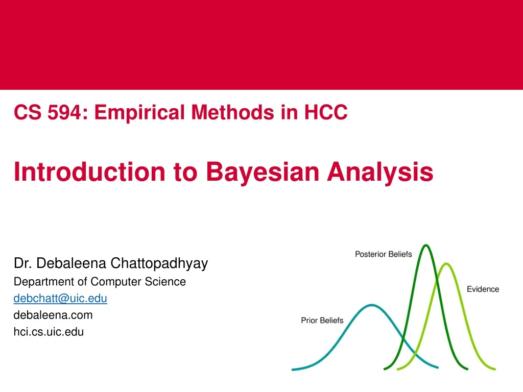
12. Steps of Bayesian Data Analysis • Identify the data relevant to RQs. Which data variables are to be predicted, and which data variables are supposed to act as predictors? • Define a descriptive model for the relevant data. The mathematical form and its parameters should be meaningful and appropriate to the theoretical purposes of the analysis. • Specify a prior distribution of the parameters. • Use Bayesian Inference to re-allocate credibility across parameter values. Interpret and check that the posterior distribution is meaningful. • Posterior predictive check: Check that the posterior predictions mimic the data with reasonable accuracy. If not, then consider a different descriptive model.

13. Parameter Estimation

14. Posterior Belief Distribution • Posterior = Likelihood * Prior / Evidence

15. High Density Interval (HDI) • HDI is formed from the posterior distribution after observing the new data. Since HDI is a probability, the 95% HDI gives the 95% most credible values. It is also guaranteed that 95 % values will lie in this interval unlike C.I.