Download
1 / 37
390 likes | 664 Views
Wavelet Applications. Texture analysis&synthesis. Compression and Coding The good approximation properties of wavelets allow to represent reasonably smooth signals with few non-zero coefficients efficient wavelet based coding systems DWT (critically sampled) Among the most famous are

E N D
Wavelet Applications Texture analysis&synthesis Gloria Menegaz
Compression and Coding The good approximation properties of wavelets allow to represent reasonably smooth signals with few non-zero coefficients efficient wavelet based coding systems DWT (critically sampled) Among the most famous are Embedded Zerotree Wavelet (EZW) Layered Zero (LZ) Coding Embedded Block Coding (EBCOT) Image denoising Image quality assessment Signal analysis The good spatial and frequency domain localization properties make wavelet a powerful tool for characterizing signals DWF (overcomplete) Feature extraction Pattern recognition Identification of structures in natural images Curvelets, ridgelets Identification of textures Classification Segmentation Wavelet based IP Gloria Menegaz
Textures Gloria Menegaz
What is texture? • No agreed reference definition • Texture is property of areas • Involves spatial distributions of grey levels • A region is perceived as a texture if the number of primitives in the field of view is sufficiently high • Invariance to translations • Macroscopic visual attributes • uniformity, roughness, coarseness, regularity, directionality, frequency [Rao-96] • Sliding window paradigm Gloria Menegaz
Statistical methods Textures as realizations of an underlying stochastic process Spatial distributions of grey levels Statistical descriptors Subband histograms, co-occurrence matrices, autocorrelation, n-th order moments, MRFs... A-priori assumptions locality, stationarity, spatial ergodicity, parametric form for the pdf (Gaussian) Structural methods Texture as sets of geometric structures Descriptors primitives+placement rules Suited for highly regular textures Feature extraction for texture analysis • Multi-scale methods • Combined with statistical methods • Models of early visual processes • Multi-resolution analysis (wavelet based) • Gabor wavelets are optimal as they have maximum resolution in space and frequency Gloria Menegaz
Texture analysis • Texture segmentation • Spatial localization of the different textures that are present in an image • Does not imply texture recognition (classification) • The textures do not need to be structurally different • Apparent edges • Do not correspond to a discontinuity in the luminance function • Texture segmentation → Texture segregation • Complex or higher-order texture channels Gloria Menegaz
Texture analysis • Texture classification (recognition) • Hypothesis: textures pertaining to the same class have the same visual appearance → the same perceptual features • Identification of the class the considered texture belongs to within a given set of classes • Implies texture recognition • The classification of different textures within a composite image results in a segmentation map Gloria Menegaz
Texture Classification • Problem statement • Given a set of classes {ωi, i=1,...N} and a set of observations {xi,k ,k=1,...M} determine the most probable class, given the observations. This is the class that maximizes the conditional probability: • Method • Describe the texture by some features which are related to its appearance • Texture → class →ωk • Subband statistics →Feature Vectors (FV) →xi,k • Define a distance measure for FV • Should reflect the perceived similarity/dissimilarity among textures (unsolved) • Choose a classification rule • Recipe for comparing FV and choose ‘the winner class’ • Assign the considered texture sample to the class which is the closest in the feature space Gloria Menegaz
Exemple: texture classes ω1 ω2 ω3 ω4 Gloria Menegaz
FV extraction • Step 1: create independent texture instances Training set Test set Gloria Menegaz
Feature extraction • Step 2: extract features to form feature vectors subimages Intensity image DWT/DWF • The FVs contain some statistical parameters evaluated on the subband images • estimates of local variances • histograms For each sub-image For each subband Calculate the local energy (variance) Fill the corresponding position in the FV Collect the local energy of each sub-image in the different subbands in a vector Classification algorithm One FV for each sub-image Gloria Menegaz
Building the FV approximation d1 d3 d2 scale 1 scale 2 Gloria Menegaz
Building the FV elements of FV1 of texture 1 elements of FV2 of texture 1 approximation d1 d3 d2 FV1 FV2 scale 1 scale 2 Gloria Menegaz
Implementation • Step 1: Training • The classification algorithm is provided with many examples of each texture class in order to build clusters in the feature space which are representative of each class • Examples are sets of FV for each texture class • Clusters are formed by aggregating vectors according to their “distance” • Step 2: Test • The algorithm is fed with an example of texture ωi(vector xi,k) and determines which class it belongs as the one which is “closest” Build the reference cluster Training set Sample Feature extraction Classification core Test set Gloria Menegaz
Clustering in the Feature Space Bi-dimensional feature space (FV of size 2) Multi-dimensional feature space FV(1) FV(1) FV(2) FV(3) FV(2) FV classification: identification of the cluster which best represents the vector according to the chosen distance measure Gloria Menegaz
Classification algorithms • Measuring the distance among a class and a vector • Each class (set of vectors) is represented by the mean (m) vector and the vector of the variances (s) of its components the training set is used to build m and s • The distance is taken between the test vector and the m vector of each class • The test vector is assigned to the class to which it is closest • Euclidean classifier • Weighted Euclidean classifier • Measuring the distance among every couple of vectors • kNN classifier Gloria Menegaz
kNN classifier • Given a vector v of the test set • Take the distance between the vector v and ALL the vectors of the training set • (while calculating) keep the k smallest distances and keep track of the class they correspond to • Assign v to the class which is most represented in the set of the k smallest distances 0.10.570.91.22.5 2.77 3.14 0.1 6.10 7.9 8.4 2.3 k=3 v v is assigned to class 1 FV for class 1 FV for class 2 FV for class 3 Gloria Menegaz
Confusion matrix Gloria Menegaz
Texture Segmentation • Problem statement • Given an image, identify the regions characterized by different features • How? • Same approach used for classification • Key difference: focus on feature gradients, namely local discontinuities in feature space represented by differences in feature vectors • If feature vectors are collections of local variances, it is the difference in such a parameter that is assumed to reveal the presence of an apparent edge • Noteworthy • More in general, segmentation is based on image interpretation, which is very difficult to model • Often “supervised” • Tailored on the application: no golden rule for segmentation! • Key point: image interpretation and semantics Gloria Menegaz
Relation to complex texture channels • Model for pre-attentive texture segregation • LNL (linear-non linear-linear) model • The idea is to detect low spatial frequency features of high spatial frequency first-stage responses [Landi&Oruc 2002] Second order linear spatial filter First order linear spatial filter Point-wise non linearity Pooling and decision Gloria Menegaz
Example of a segmentation map texture1 texture 2 texture 3 texture 4 texture 5 texture 6 texture 7 texture 8 texture 9 texture 10 Gloria Menegaz
Define a generative model to create new textures having the same visual appearance of the original one Stochastic methods Reproduce statistical descriptors Co-occurrence matrices, autocorrelation features, MRF Very natural Could require parameter estimation Usually high computational cost Structural methods Crystal growth Highly structured and regular textures Texture synthesis • Multi-scale methods • Reproduce Intra-band and Inter-band relationships among subband coefficients • pixel statistics,subband marginals and covariance, subband joint distributions • Explicit or Implicit • Suitable for both natural and artificial structured textures Gloria Menegaz
Recipe for perceptual texture synthesis • Consider the image as a realization of an underlying stochastic process • Define a stochastic model for the stimulus as well as criterion for sampling from the corresponding distribution and generating a new realization • Possible approaches • Parametric techniques: explicit constraining of statistical parameters • Filters Random fields And Maximum Entropy (FRAME) model [Zhu&Mumford-05] • Constraining Joint statistics of subband coefficients [Portilla&Simoncelli-00] • Non parametric techniques • Multi-resolution probabilistic texture modeling [De Bonet-97] • DWT based non parametric texture synthesis [Menegaz-01] Gloria Menegaz
Portilla&Simoncelli • Statistical parameters • Marginal and joint subband statistics • Variance and other 2nd order moments • Auto and mutual correlations between subbands • Magnitude correlations →non-linearity • Self and mutual correlations between phase images Reference model (statistics of the original sample) Constraining subband statistics Multi-scale oriented decomposition (Wavelet transform) Gloria Menegaz
Portilla&Simoncelli Gloria Menegaz
DWT based texture synthesis • Controlled shuffling of hierarchies of wavelet coefficients Original sample model MRA Multi-scale conditional sampling Inverse transform (reconstruction) Perceptual testing Synthesized sample Gloria Menegaz
Multiresolution Probabilistic TM original sample Perceptual decomposition Multiscale orientation-selective decomposition mimicking the neural responses to the visual stimulus Non-parametric constraining of the joint distributions of subband coefficients. Inter-band dependencies among subbands with same orientation at different scales are preserved by multiscale conditional sampling Statistical modeling Sampling The appearance of a subband coefficient at a given scale and orientation is conditioned to the appearance of its ancestors at all coarser scales parent vector Reconstruction The synthesis pyramid is filled by sampling from the analysis pyramid, and is then collapsed to get the synthetic image synthesized sample If the resulting texture is not satisfying, the procedure is repeated with different model parameters Perceptual testing Gloria Menegaz
Formally Feature Vector (M: #feature images, N:# of levels): Gloria Menegaz
Non-parametric Model Chain across scales: Gloria Menegaz
Conditional Sampling Gloria Menegaz
Texture sample Syntesized texture LL1 HL1 LL1* HL1* LH1 HH1 LH1* HH1* DWT IDWT Conditional sampling DWT based MPTM Gloria Menegaz
MPTM results Gloria Menegaz
Generalization to 2D+1 Textures • 2D+1 textures are meant as the result of the observation of a realization of a stochastic 2D process by a moving observer • Temporal features are due to the change of the observation point of view • Key point: preserve the temporal relation between successive images in the sequence • Major issue: define a growing rule for subband regions simulating any displacement in image space • Hypothesis • The motion is given • The trajectory is piece-wise linear • Guideline • Integrate the motion information within the DWT-based Multiresolution Probabilistic Texture Modeling (MPTM) algorithm [Menegaz-00] • Advantages • Suitable for the integration in a coding system • Low complexity running in real time Gloria Menegaz
Example 1 Gloria Menegaz
Example 2 Gloria Menegaz
Example 3 Gloria Menegaz
Color Textures Textures Color distributions with a spatial structure • When different color distributions are perceptually equivalent? • How do texture and color interact? On going research Gloria Menegaz