Physical Organization Index Structures Query Processing
530 likes | 646 Views
This document explores the key issues of formatting records within blocks and fields in data processing. It delves into fixed-length and variable-length fields, indexed heaps, and the complexities of assigning records to blocks. The discussion extends to various index structures such as ISAM and B-trees, their advantages, and disadvantages. Key considerations include the implications of formatting records, the efficiency of retrieval methods, and the impact of updates on indexed data structures. Understanding these concepts is vital for effective data management and processing.

Physical Organization Index Structures Query Processing
E N D
Presentation Transcript
Physical OrganizationIndex StructuresQuery Processing Vishy Poosala
Ke y issues • (1) Formatting fields within a record • (2) Formatting records within a block • (3) Assigning records to blocks.
Formatting fields within a record. • Fixed length fields stored in a specific order. • Fixed length fields stored as an indexed heap. • Fields need not be stored in order. • There is exactly one pointer in the header for each field, whether it is present or not. • Variable length fields delimited by special symbols or length.
Formatting records within a block. • Fixed-packed: The records are stored contiguously within the block. • A record is located by a simple address calculation. • The structure is highly inflexible and introduces inefficiencies. • * Records may span blocks (expensive). • * Insertion and deletion become complicated. • * Page reorganization affects external pointers.
Indexed heap • A block header contains an array of pointers pointing to the records within the block. • A record is located by providing its block number and its index in the pointer array in the block header. • The combination of block number and index is called TID.
Insertion and deletion are easy; they are accomplished by manipulating the pointer array. • The block may be reorganized without affecting external pointers pointing to records, i.e., records retain their tid even if they are moved around within a block
Assigning records to blocks. • Heap: Records are assigned to blocks arbitrarily, more or less in the order of insertion. • easy to maintain but provides no help for retrievals whatsoever • Keyed placement: Records are assigned to blocks according to the values of some key fields. • The supporting structure implementing the mapping of records with specific values in the key fields to blocks is called an index.
Keyed placement • This facilitates the execution of retrievals, since to a large extent, only relevant records are retrieved. • Updates (insertions and deletions) become more expensive, because of the index maintenance. • There are three major index structures: • * Hashing • * B-trees • * ISAM
Keyed placement by sorting • Sort the file on the key field(s). • It is a special case of the general keyed placement, with the distinguished characteristic that there is no index to be supported. • Retrievals are performed by binary search • Faster equality selection than nonkeyed. • Good for range queries, e.g., age between 22 and 28. • Efficient joins, applying merge-scan. • Slower equality selection than other keyed index structures. • Updates are a pain.
Index Structures - ISAM • ISAM is a multilevel tree structure providing direct access to tuples in a relation sorted according to some attribute. • That attribute is called the key of the structure.
Each node of the tree is a page (block) on the disk. The nodes of the tree contain <key_value,pointer> pairs, sorted on key_value. • The internal nodes point to lower nodes in the tree, whereas the leaf nodes point to pages in the relation. • A pointer points to a subtree with key values greater than or equal the corresponding key_value and less than the key_value corresponding to the next pointer.
Comments • The tree structure is static, i.e., the key_values in the internal nodes do not change as tuples are inserted into the relation. • To accommodate insertions of new tuples, overflow pages are created in the relation forming a linked list. • Usually, tuples within the linked list of the primary and overflow pages are not sorted.
Comments • Occasionally, the index is created with the nodes filled at less than maximum capacity in anticipation of future updates. • Excessive overflows result in highly unbalanced trees. In this case, the relation is sorted and the index is created again.
Advantages of ISAM • It provides a directory for a relation that is (for the most part) sorted. Exact queries on the key values, e.g., salary=30K, are much faster than for an unstructured relation. • The system starts at the root of the tree. It follows the pointers down the tree according to the given value, until it finally reaches a data page in the relation. • It scans sequentially the data page and the possible overflow pages and gets the tuples satisfying the qualification.
Assume that there are no overflow pages. Why is ISAM better than binary search on the relation? • Why is ISAM better than binary search on a 1-level index? • Costs of 4 methos: • Scan, Binary search, Binary search on 1-level index, and ISAM. • ISAM also facilitates the execution of range queries, e.g., 20K<=salary<=40K
Disadvantages • It is a static structure and may get unbalanced. • If there is a lot of update activity the relation may be far from being "nearly sorted". • The index does consume some space, which in some cases is valuable.
B+-Trees • Most popular Index structures • Like ISAM • multi-level tree structure • sequential data organization below • supports range, equality predicates • But, Better • never gets unbalanced • dynamic reorganization
Leaf nodes contain tuples in sorted order and are connected in that order • All other internal nodes are of the following form: • [P_1, K_1, P_2, K_2, ..., P_(N-1), K_(N-1), P_N] • say, [...s_i, p_i, k_(i+1),...] is the parent node • P_1 points to a node containing key values v, v < K_1; v >= s_i • P_2 points to: K_1 <= v < K_2; .. • P_N points to: v >= K_(N-1), v <s_(i+1)
Every node is a page • The data structure is on disk • Each useful node is brought into memory for processing • Operations within a page are done in memory
B+Tree Searching • Follow pointers down the tree, looking for the given value. • Input: Key value v. Output: Node containing tuple with key value v. • Node := Root; • While (Node is not a leaf) do • Find i s.t. K_(i-1) <= v < K_i in Node; • Node := P_i; • end • Print (Node);
B+tree updates • The tree has to remain balanced on updates in order for the fast access • To insert a tuple with key value v, search for the leaf on which v should appear. • If there is space on the leaf, insert the tuple. • If not, split the leaf in half, and split the range of keys in the parent node in half also. • If the parent node was also full, split that one. If this propagates to the root, split the root also.
B+Tree- Deletes • To delete a tuple with key value v, search for the leaf on which v should appear and delete it • If after the record is deleted the leaf becomes less than half full, then either • move records into adjacent nodes, delete the leaf, and propagate the deletions to the parent, or • move records from adjacent leaves into the underflowed leaf and propagate the changes.
B-Trees • They have pointers to data from the internal nodes. • For each key value that appears in an internal node, there is a direct pointer from that node to the leaves with tuples with that key value. • Advantages: Occasionally faster, if the key values are found early. • Disadvantages: Trees tend to be deeper because of the smaller fanout. The implementation is also more difficult.
Hashing • Hashing Divide the set of blocks of the relation into buckets. Often each block is a bucket. • Select the field(s) which is (are) being indexed. • Devise a hashing function which maps each value in the field into a bucket.
V: Set of field values • B: The number of buckets H • The hashing function H: V -> {0,1,2,...,B-1} • Example: • V: 9 digit SSN • B: 1000 • H: V -> {0,1,2,...,999} • H(v) = last 3 digits of v = v MOD 1000 • Almost any numeric function that generates "random" numbers in the range of [0,B-1] is feasible.
One of the most popular hashing functions is MOD, i.e., divide the field value by B and interpret the remainder as the bucket number. • Example • What is a BAD Hash function? Why? • Overflows
Overflows can occur because of the following reasons: • Heavy loading of the file. • Poor hashing function, which doesn't distribute field values uniformly. • Statistical peculiarities, where too many values hash to the same bucket.
Overflows are usually handled by one of the following ways. • Chaining: If a bucket fills up, chain an empty block to the bucket to expand it. • Open Addressing: If H(v) is full, store the record in H(v)+1, and so on. • Two Hashing Functions: If H(v) is full try H’(v). If that is full, try any of the above solutions.
Performance of a hashing scheme depends on the value of the loading factor = (# tuples in the relation) / (B x S), where B= # buckets S= # tuples/bucket • Rule of thumb: When loading factor becomes too high, a typical tactic is to double B and rehash
Good/Bad • Hashing is great for exact queries • Since hashing doesn't keep the tuples in any sorted order, it is no help with range queries.
Secondary Indices • The B+trees we looked at so far are primary indexes • i.e., data is sorted in the order of the index key. • Unless tuples are stored redundantly, a file can only have at most one primary index • To improve performance of value-based queries on other fields, secondary indices can be constructed that point to tuples in the file, not necessarily stored in order.
Example • Primary B+tree index of Emp(name, sal, age) on sal; and secondary hash index on age.
Query Processing • Architecture of a DBMS query processor • query language compiler translates the query into an internal form, usually a relational algebra expression • query optimizer examines all the equivalent algebraic expressions and chooses the one that is estimated to be the cheapest. • code generator or the interpreter implements the access plan generated by the optimizer
access methods support commands to access records of a file, one at a time • Record layout on pages • Field layout in records • Indexing records by field value • file system supports page-at-a-time access to files. • Partitioning the disk into files • Managing free space on disk • Issuing hardware I/O commands • Managing main memory buffers.
Query optimization • Given a query Q, there is a set A of access plans (strategies) to execute Q and find the answer. • Query optimization is a process of identifying the access plan with minimum cost. • What access plans are there? • How do we compute a plan’s cost? • How do we pick the best choice access plan?
Query Cost Estimation • The cost is usually a weighted sum of the I/O cost (number of page accesses) and CPU cost (msec's). • Parameters the optimizers use to estimate execution costs: • p(R) For a relation R, its size in pages. • t(R) For a relation R, its size in tuples. • v (A, R) For an attribute A in relation R, the number of unique values in A • min (A, R) For an attribute A in relation R, the minimum value in A. And max(A,R) • s(f) Selectivity of the operator f
Selectivity • Ratio of result size to product of input sizes • Why? • Need to know sizes of intermediate result sizes • For estimating their costs
Assumptions • To start with: access plans don’t use indices • ignore CPU costs. • Make uniform distribution assumption over the data
Access Plans - Selections • scan the entire file • get tuples in memory • apply predicate • Cost = p(R) • Selectivity: • equality predicate (A = c): t(R) / v(A) • range predicate (A > c): t(R) * (max(A,R)-c) / (max(A,R)-min(A,R))
Access Plans - Nesed Loop Joins • The system scans the complete relation R (outer loop). • For each tuple in R, it scans S (inner loop) and whenever the tuples in S and R match on join attribute, their combination is put in the result. • for each r in R do • for each s in S do • if r.A=s.A then put s,~r in the result
N-L Join • Estimated cost (with one buffer page per relation): p ( R ) + t(R) * p (S) • Estimated cost for page nested loops (scan the inner relation once for every page of the outer relation): p ( R )+ p(R) * p ( S ) • Estimated size of result (assume the same number of unique values in A in both relations): (1/ v( A, R)) t(R) t(S)
Merge Scan / Sort Merge Join • The system sorts R and S on the join attribute A (if they are not already sorted). • It then scans the two sorted relations in parallel, merging tuples with matching join attribute values • Cost • sortcost(R) + sortcost(S) + p(R) + p(S) • Result Size: same as NL
Projection • Scan the relation • Select out the necessary attributes • Cost: p(R)
Sorting • Internal sorting doesn’t work very well • data doesn’t fit in memory • Need external sorts • Use k-way merge sort
2-way merge sort • Consider a relation R with p(R) pages and w buffer pages (Assume that p(R)/w = 2^k ) • Read in, sort in main-memory, and write out chunks of w pages. (2^k sorted chunks of w pages.) • Read in, merge in main-memory, and write out pairs of sorted chunks of w pages. (2^(k-1) sorted chunks of 2w pages.)
2-Way External Sort • Read in, merge in main-memory, and write out pairs of sorted chunks of 2w pages. (2^(k-2) sorted chunks of 4w pages.) • ... • Read in, merge in main-memory, and write out pairs of sorted chunks of 2^(k-2)w pages. (2 sorted chunks of 2^(k-1)w pages.) • Read in, merge in main-memory, and write out pairs of sorted chunks of 2^(k-1)w pages. (1 sorted chunk of 2^kw = p(R) pages.)
Cost of External Sort • Each pass requires reading and writing of the whole file. The algorithm's I/O cost • is c(2-way sort ) = 2 p(R) (k+1) = 2 p(R) [log (p(R)/w) + 1 ] • Example: Sort a 20-page relation having a 5-page buffer pool. • Exercise: can do 3-way sort, 4-way, ..., (w-1)way! • They are cheaper.
Query Processing with Indexes • Cost = Cost(index) + Cost(data) • New parameters: • p(I) For an index I, its size in pages. • d(I) For a tree index I, the depth of the tree. • lp(I) For a tree index I, the number of leaf pages. • B(I) For a hash index I, the number of buckets
Selection (A = c) • Heap: P(R) • Hash (primary): P(R) / B(I) • Hash (secondary): P(I) / B(I) + t(R)/v(A,R) • B-tree (primary): d(I) + P(R) / v(A,R) • B-tree (secondary): d(I) + lp(I)/v(A,R) + t(R) / v(A,R)
Selection (A >= c) • Heap: P(R) • Hash (primary, secondary): P(R) • B-tree (primary): d(I) + frac(c) * P(R) • frac(c) = (max(A,R) - c) / (max(A,R) - min(A,R)) • B-tree (secondary): d(I) + frac(c) * lp(I) + frac(c) * t(R)
