Download
1 / 17
180 likes | 305 Views
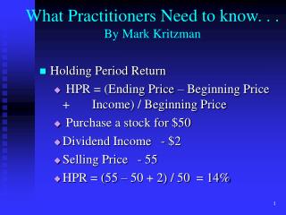
What Practitioners Need to know. . . By Mark Kritzman. Holding Period Return HPR = (Ending Price – Beginning Price + Income) / Beginning Price Purchase a stock for $50 Dividend Income - $2 Selling Price - 55 HPR = (55 – 50 + 2) / 50 = 14%. Dollar Weighted vs. Time Weighted.

E N D
What Practitioners Need to know. . .By Mark Kritzman • Holding Period Return • HPR = (Ending Price – Beginning Price + Income) / Beginning Price • Purchase a stock for $50 • Dividend Income - $2 • Selling Price - 55 • HPR = (55 – 50 + 2) / 50 = 14%
Dollar Weighted vs. Time Weighted • Rate of Return over multiple holding periods. Assume the annual holding period returns for mutual funds. • Total Investment = $75,000 • Ending Value = $103,804.56
Dollar Weighted Return • Dollar weighted return is the same as IRR. • 5000 = -10,000/(1+r) – 15,000/(1+r)^2 - …. - 25,000/(1+r)^4 + 103,805 / (1+r)^5 • r = 14.25% • If the contribution is reversed: • 25,000 = -20,000/ (1+r) – 15,000 / (1+r)^2 -….+ 103,8905/(1+r)^5 • r = 9.12%
Time Weighted Rate of Return • Same as Geometric Return • Return is wealth relative • TWR = [n i=1 (1 + HPRi ) ]1/n – 1 • Example: • Invest $10,000; Year 1 HPR = 50%; • Year 2 HPR = -50% ; Ending wealth = $7,500 • TWR = [(1+.5)(1-.5)]1/2 – 1 = -13.4%
Time Weighted Rate of Return • Arithmetic Return for the same example is: [(50%) + (-50%)] / 2 = 0% • Arithmetic Return always exceeds Geometric Return. Overestimates performance. Most studies dealing with long-term historical performance include both arithmetic and geometric rates of return.
Application of Geometric Return FV20 Example: You expect to receive a geometric return of 8% over a 20 year horizon. During the past 5 years, the fund’s geometric return had been 6.5%. What must its geometric return be for the remaining 15 year if you are to meet your original goal? 8% 6.5% r = ? FV 20 PV 5 Yr 8%
Application of Geometric Return • At 8% FV20 = $1,000(1.08) 20 = $466,095.7 • 20 year 8% intent factor = 4.66095 • 5 year 6.5% intent factor = 1.37008 • 15 year return = (4.66095 /1.37008)1/15 – 1 = 8.5%
What Practitioners Need to know about Uncertainty? • Define Risk vs. Uncertainty • Random variable (Stock Price): an event whose outcome in a given situation depends on chance factors. Because an outcome is influenced by chance does not mean that we are completely ignorant about its possible values.
RISK (Contd.) • We are interested in predicting the return of S&P 500 over the next 12 months. • Should it be between 0 and 10% than 10 to 20%? • Consider Table 1: Raw data of S&P500 Return
RISK (Contd.) Table 2: Relative frequency = Frequency / Frequency • 24/40 (~ 2/3) more likely to observe a return within the range of 10 to 20% than a return within the range of 0 to 10% • 25% chance of experiencing a negative return
Normal Distribution • Continuous probability distribution – infinite number of observations covering all possible values along a continuous scale. • [Stock Price is quoted as 1/8th, therefore it cannot have a continuous scale] • Normal Distribution is a normal approximation for stock price movement.
Normal Distribution (Contd.) • Normal Distribution can be described fully by two values: • Mean of the observations • Variance of observations • Mean = or 12.9% from Table 1 2. 2 = = 2.9% ; S.D = 16.9% Explain Figure B: S.D. = 12.9 (1) (16.9)
Standardized Variable A) Likelihood of experiencing a return of less than 0% or greater than 15%. • In order to determine the probabilities of these returns, we can standardize the target return. • Standardized returns have zero mean and a SD of 1 • Standardized Value =(0%-12.9%)/16.9% = -0.7633
Standardized Variable • 0% is 0.7633 SD below mean • How to read Standard Normal Table • To find the area under the curve to the left of standardize variable. The probability of experiencing a return less than 0% is .2236. • Therefore the chance of experiencing return greater than 0% is (1- .2236) = .7764%
Standardized Variable (Contd.) B) To find the likelihood of experiencing an annualized return of less than 0% on average over a five year horizon. (Assume year- by- year return is independent) • = = -1.71 • Using the Standardized Normal Table • = .0436 = 4.36%
Standardized Variable (Contd.) C)Likelihood that we might lose money in one or more of the five years: • This probability is equivalent to = • (1 – Probability of experiencing a positive return in every one of the five years) • Previously obtained: Probability of experiencing a return greater than 0% = .7764
Standardized Variable (Contd.) • Likelihood of experiencing five consecutive yearly return each greater than 0% = (.7764)5 = .2821 • Probability of experiencing a negative return in at least one of the five years = (1 - .2821) = .718