Download
1 / 20
200 likes | 349 Views
Mapping of arid regions in N. Africa, middle East and Southeast Asia using VGT S10. Michael Cherlet. Mapping of arid regions in N. Africa, middle East and Southeast Asia using VGT S10. Photo from 300 m height. Mapping of arid regions in N. Africa, middle East and Southeast Asia using VGT S10.

E N D
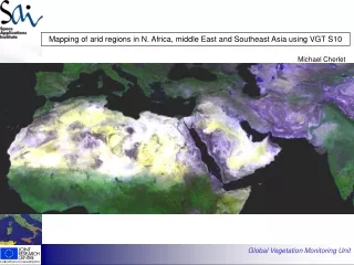
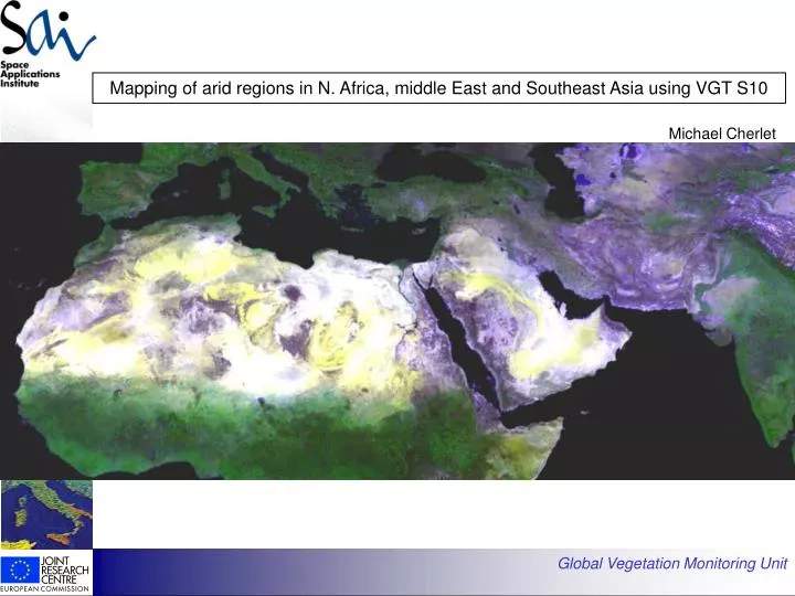
Mapping of arid regions in N. Africa, middle East and Southeast Asia using VGT S10 Michael Cherlet Global Vegetation Monitoring Unit
Mapping of arid regions in N. Africa, middle East and Southeast Asia using VGT S10 Global Vegetation Monitoring Unit
Photo from 300 m height Mapping of arid regions in N. Africa, middle East and Southeast Asia using VGT S10 Global Vegetation Monitoring Unit
Specific Problematic for Mapping Land Cover in Arid Areas Low cover vegetation >> 3% - 40% (LCCS: sparse to open) mixed with background soil S10 NDVI products >> high variability of NDVI not explained only by vegetation Global Vegetation Monitoring Unit
IGBP Global Vegetation Monitoring Unit
Specific Problematic for Mapping Land Cover in Arid Areas timing ofseasonal variability related to vegetation is difficult to determine: - erratic character of rainfall in space and time - influence of two climatic zones N > Mediterranean influence S > ‘tropical’ ITCZ influence not possible to ‘choose’ best period for vegetation development throughout year >> difficult to use S1 Global Vegetation Monitoring Unit
Specific Problematic for Mapping Land Cover in Arid Areas Using SPOT VGT S10 or longer composites based on MVC: atmospheric, aerosol or clouds contamination is limited in S10 over arid areas (no persistence) BRDF effect which is probably ‘enhanced’ in relation to topography Spectral behaviour related to lithology and geology (colour) confusion between low cover vegetation and sandy soils/sand-stones Global Vegetation Monitoring Unit
Oct dek 1: Unsure: 0.505 % of image Cloud :0.059 % of image Nov dek 1: Unsure: 0.715 % of image Cloud :0.029 % of image Nov dek 2: Unsure: 0.915 % of image Cloud :0.009 % of image Contamination on S10 Threshold on ratio MIR/BO improves classification of unsure class Global Vegetation Monitoring Unit
Specific Problematic for Mapping Land Cover in Arid Areas Using SPOT VGT S10 or longer composites based on MVC: atmospheric, aerosol or clouds contamination is limited over arid areas (no persistence) BRDF effect which is probably ‘enhanced’ in relation to topography Spectral behaviour related to lithology and geology (colour) confusion between low cover vegetation and sandy soils/sand-stones Global Vegetation Monitoring Unit
16 26 12 10 23 24 31 8 25 30 3 2 4 29 13 14 15 21 7 11 5 20 9 Backward Foreward NDVI In general, but locally of importance increases confusion of e.g. sandstone outcrops and vegetation Global Vegetation Monitoring Unit
Specific Problematic for Mapping Land Cover in Arid Areas Using SPOT VGT S10 or longer composites based on MVC: atmospheric, aerosol or clouds contamination is limited over arid areas (no persistence) BRDF effect which is probably ‘enhanced’ in relation to topography Spectral behaviour related to lithology and geology (colour) confusion between low cover vegetation and sandy soils/sand-stones Global Vegetation Monitoring Unit
0.36 =~ 40% NDVI 0.786 = 100% Final Approach still open Three methods tried: 1. 1.producing yearly composites: - NDVI image Max, Min, amplitude + statistics (st. dev….) (cloudmask) - NDWI image Max, Mean, Min, amplitude + statistics (#methods tested) - Minimum B0, B2, B3, Mir differentiation of different zones/masks using Max NDVI thresholds (~ cover) Sensor sensitivity: 0.01 Global Vegetation Monitoring Unit
- non-supervised classification (isoclass) within masks using yearly derived products - grouping of ‘non-vegetation’ vs ‘vegetation’ classes and re-iterate isoclass and regrouping (min 3) based on subjective interpretation of all available data and field knowledge - final grouping of all ‘non-vegetation’ and ‘vegetation’ masks - differentiation of a. physical features using isoclass on bands and regrouping within ‘non-vegetation’ b. different ‘life forms’ within ‘vegetation’ part using NDVI time series statistics and ancillary data Global Vegetation Monitoring Unit
IGBP IGBP Orange: 3 - 6 % cover (GP length?) > LCCS: sparse herbaceous Aquam: 6 - 10 % cover (GP length?) > LCCS: herbaceous green1: 10 - 20 % cover (GP length?) > LCCS: green2: 20 - 40 % cover (GP length?) > LCCS: Global Vegetation Monitoring Unit
2. 2. - producing yearly composites: - NDVI image Max, Min, amplitude + statistics (st.dev….) - NDWI image Max, Mean, Min, amplitude + statistics - Min B0, B2, B3, Mir - stratification of land-units based on classification of bands (isoclass and re-grouping) - non-supervised classification (isoclass) within landunits using yearly derived products - grouping of ‘non-vegetation’ vs ‘vegetation’ classes and re-iterate isoclass and regrouping (min 3) based on subjective interpretation of all available data and field knowledge - final grouping of all ‘non-vegetation’ and ‘vegetation’ masks - differentiation of a. physical features using isoclass on bands and regrouping within ‘non-vegetation’, = optimizing first stratification b. different ‘life forms’ within ‘vegetation’ part using NDVI time series statistics and ancillary data Used to attach further info to vegetation classes: Global Vegetation Monitoring Unit
(Using Gaussian density probability function) Decreasing weight with increasing NDVI value above the mean Difference less than1% the process stops 1st average - weight=1 2nd average - weight=GF Δ Same weight (1) for the NDVI values under the mean 3. 3. Determination of ‘vegetation’ character of individual pixels based on detection of significant NDVI change during year 2000 by separation of ‘background noise’ from ‘signal’ using long term time series to establish ‘noise’ level per pixel (*): Global Vegetation Monitoring Unit (*) in cooperation with Univ. UCL, Belgium
Image of MEAN of ‘dry’ season Image of STANDARD DEVIATION of dry season Result of the iterative process Pixel FLAGGED NDVI > Mean + nSTD Reflects a status of CHANGE in ‘probable’ vegetation cover related to its “dry season” status (whatever that is .... Soil or vegetation....) Global Vegetation Monitoring Unit (*) in cooperation with Univ. UCL, Belgium
Avg + 2*STdev Global Vegetation Monitoring Unit
Temporal mask …… and spatial mask Needs refining to be used as base “probable vegetation” - non vegetation Global Vegetation Monitoring Unit
Conclusions: methods 1 & 2 - straightforward techniques - need for ‘ground’ knowledge - subjective - not very repeatable method 3 - still to be validated technique - fine tuning required - objective - repeatable - ‘ground’ knowledge only required in final stage Global Vegetation Monitoring Unit