Section 6.4
Section 6.4. Normal Approximation to the Binomial Distribution. Focus Points. State the assumptions needed to use the normal approximation to the binomial distribution. Compute and for the normal approximation.


Section 6.4
E N D
Presentation Transcript
Section 6.4 Normal Approximation to the Binomial Distribution
Focus Points • State the assumptions needed to use the normal approximation to the binomial distribution. • Compute and for the normal approximation. • Use the continuity correction to convert a range of r values to a corresponding range of normal xvalues. • Convert the x values to a range of standardized z scores and find desired probabilities.
Normal Approximation to Binomial Distribution • The probability that a new vaccine will protect adults from cholera is known to be 0.85. The vaccine is administered to 300 adults who must enter an area where the disease is prevalent. • What is the probability that more than 280 of these adults will be protected from cholera by the vaccine? • This question falls into the category of a binomial experiment, with the number of trials n equal to 300, the probability of success p equal to 0.85, and the number of successes r greater than 280.
Normal Approximation to Binomial Distribution • It is possible to use the formula for the binomial distribution to compute the probability that r is greater than 280. • However, this approach would involve a number of tedious and long calculations. • There is an easier way to do this problem, for under the conditions stated below, the normal distribution can be used to approximate the binomial distribution.
Example 11 – Binomial distribution graphs • Graph the binomial distributions for which p = 0.25, q = 0.75, and the number of trials is first n = 3, then n = 10, then n = 25, and finally n = 50. • Solution: • The authors used a computerprogram to obtain the binomialdistributions for the given valuesof p, q, and n. The results havebeen organized and graphedin Figures 6-34, 6-35, 6-36, and 6-37. Figure 6-34
Example 11 – Solution cont’d Figure 6-35 Figure 6-36 Good Normal Approximation; np > 5 and nq > 5 Figure 6-37
Example 11 – Solution cont’d • When n = 3, the outline of the histogram does not even begin to take the shape of a normal curve. But when n = 10, 25, or 50, it does begin to take a normal shape, indicated by the red curve. • From a theoretical point of view, the histograms in Figures 6-35, 6-36, and 6-37 would have bars for all values of r from r = 0 to r = n. • However, in the construction of these histograms, the bars of height less than 0.001 unit have been omitted—that is, in this example, probabilities less than 0.001 have been rounded to 0.
Example 12: Normal Approximation • The owner of a new apartment building must install 25 water heaters. From past experience in other apartment buildings, she knows that Quick Hot is a good brand. A Quick Hot heater is guaranteed for 5 years only, but from the owner’s past experience, she knows that the probability it will last 10 years is 0.25. • (a) What is the probability that 8 or more of the 25 water heaters will last at least 10 years? Define success to mean a water heater lasts at least 10 years.
Example 12: Normal Approximation • Solution: • Using the binomial distribution (see Figure 6-36) n = 25, p = 0.25, P(r ≥ 8) = 1 − binomcdf(25, 0.25, 7) = 0.2735 • (2) Using normal distribution μ = np = 25(0.25) = 6.25, q = 0.75 σ ≈ 2.17 (square root of npq) x = 8 − 0.5 = 7.5 z ≈ 0.576 P(x ≥ 7.5) = P(z ≥ 0.576) = 0.2823
Example 12: Normal Approximation • (b) How does this result compare with the result we can obtain by using the formula for the binomial probability distribution with n = 25 and p = 0.25? • (c) How do the results of parts (a) and (b) compare?The error is negligible.
Normal Approximation to Binomial Distribution • Procedure:
Normal Approximation to Binomial Distribution P(6 r 10) Is Approximately Equal to P(5.5 x 10.5) Figure 6-38
Guided Exercise 12 • From many years of observation, a biologist knows that the probability is only 0.65 that any given Arctic tern will survive the migration from its summer nesting area to its winter feeding grounds. A random sample of 500 Arctic terns were banded at their summer nesting area. Use the normal approximation to the binomial and the following steps to find the probability that between 310 and 340 of the banded Arctic terns will survive the migration. Let r be the number of surviving terns. • (a) To approximate P(310 ≤ r ≤ 340), we use the normal curve with μ = ________ and σ = ________.μ = np =325, σ ≈ 10.67
Guided Exercise 12 • (b) P(310 ≤ r ≤ 340) is approximately equal to P(______ ≤ x ≤ ______), where x is a variable from the normal distribution described in part (a).P(309.5 ≤ x ≤ 340.5) • (c) Convert the condition 309.5 ≤ x ≤ 340.5 to a condition in standard units.-1.4527 ≤ z ≤ 1.4527
Guided Exercise 12 • (d) P(310 ≤ r ≤ 340) = P(309.5 ≤ x ≤340.5) = P(−1.4527 ≤ z ≤ 1.4527) = __________.normalcdf(−1.4527, 1.4527, 0, 1) = 0.8537normalcdf(309.5, 340.5, 325, 10.67) = 0.8537 • (e) Will the normal distribution make a good approximation to the binomial for this problem? Explain your answer.Binomcdf(500, .65,340)−binomcdf(500, .65, 309) = 0.8540 • np = 500(0.65) = 35 > 5nq = 500(0.35) = 175 > 5So, good approximation.
Answers to some even hw: • 4. a) 0.159b) μ = 9; σ ≈ 2.225; 0.1615c) Difference of about 0.003 • 8. np > 5; nq > 5. μ = np = 40.32, σ ≈ 3.8099a) 0.7881b) 0.9936c) 0.7817 • 10. np > 5; nq > 5. μ = np = 40.32, σ ≈ 3.8099a) 0.9370b) 0.9842c) 0.9633d) 0.7157