Download

1 / 23
230 likes | 335 Views
This lecture explores discrete stochasticity, focusing on the binomial distribution and its properties. A stochastic test is conducted using binomial trials to observe how the distribution approaches a normal distribution as the number of trials increases. The session includes simulations of population dynamics using stochastic models, demonstrating how factors such as probability and initial conditions impact outcomes. Participants can gain insights into the mathematical principles and applications of stochasticity in real-world scenarios, emphasizing data analysis and probabilistic modeling.

E N D
CEE162/262c Lecture 13: Discrete Stochasticity CEE162/262c Lecture 13: Discrete stochasticity
c = 4 c = 3 c = 2 c = 1 c = 0 j = 0 j = 1 j = 2 j = 3 …. j = n CEE162/262c Lecture 13: Discrete stochasticity
m+1 m j j+1 CEE162/262c Lecture 13: Discrete stochasticity
%%%%%%%%%%%%%%%%%%%%%%%%%%%%%%%%%%%%%%%%%%%%%%%%%%%%%%%%%%%%%%%%%%%%%%%%%%%%%%%%%%%%%%%%%%%%%%%%%%%%%%%%%%%%%%%%%%%%%%%%%%%%%%%%%%%%%%%%%%%%%%%% % % File: jumps.m % Description: Stochastic test of the binomial distribution. % %%%%%%%%%%%%%%%%%%%%%%%%%%%%%%%%%%%%%%%%%%%%%%%%%%%%%%%%%%%%%%%%%%%%%%%% function jumps() nmax = 100; Pc = 0.04; trials = [10,100,1000,10000]; for numtrials=trials k = sum(rand(nmax,numtrials)<Pc); N = hist(k,[0:nmax])/numtrials; kt = [0:nmax]; p = choose(nmax,kt).*Pc.^kt.*(1-Pc).^(nmax-kt); sp = find(numtrials==trials); figure(1); subplot(length(trials),1,sp); plot(kt,N,'k.-',kt,p,'k:','markersize',10); if(sp<length(trials)) set(gca,'xticklabel',[]); end title(sprintf('%d trials',numtrials)); axis([0 20 0 .25]); end function c = choose(n,k) c = factorial(n)./(factorial(n-k).*factorial(k)); CEE162/262c Lecture 13: Discrete stochasticity
Binomial distribution approaches a normal distribution as n infinity. CEE162/262c Lecture 13: Discrete stochasticity
% cranes.m – Stochastic crane population simulation nmax = 5; Pc = 0.04; numtrials = 10000; x0 = 100; r = 0.4; rc = 0.175; eps = 1e-10; kfound = 0; xend = zeros(numtrials,1); for trial=1:numtrials x = x0; cs = 0; for n=1:nmax s = rand()<Pc; cs = cs + s; x = s*(1+rc)*x + (1-s)*(1+r)*x; end ct(trial) = cs; if(kfound==0) xs = x; kfound = 1; else if(min(abs(x-xs))>eps) xs = [xs,x]; kfound = kfound + 1; end end xend(trial) = x; end xs = sort(xs); [Nc,c] = hist(ct,[0:nmax]); [Nx,x] = hist(xend,xs); fprintf('# Cat.\tp(Cat.)\t\tPop.\t\tp(Pop.)\n'); for n=1:length(Nx) fprintf('%d\t\t%.4f\t\t%.0f\t\t%.4f\n',... c(n),Nc(n)/numtrials,x(n),Nx(n)/numtrials); end Output: # Cat. p(Cat.) Pop. p(Pop.) 0 0.8159 317 0.0008 1 0.1694 378 0.0139 2 0.0139 451 0.1694 3 0.0008 537 0.8159 CEE162/262c Lecture 13: Discrete stochasticity