Lecture 21
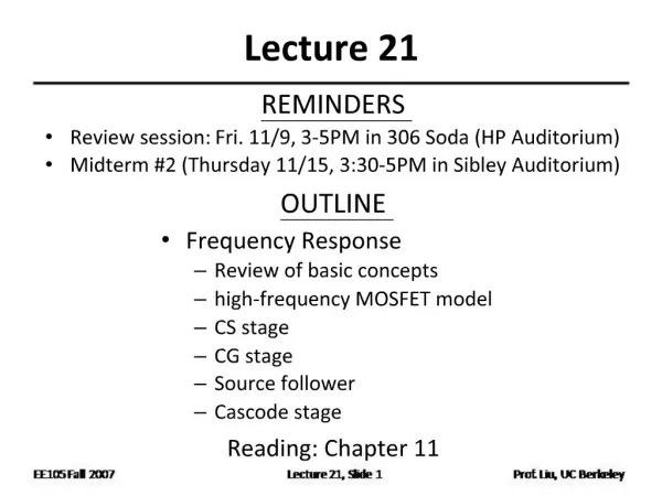
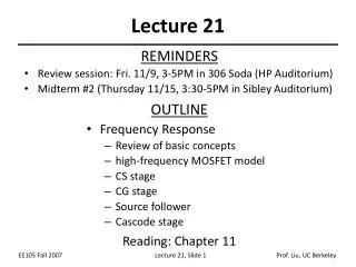
Lecture 21. MP574. Radon/Inverse Radon Simulation. Sinogram. 1D DFT. Ram-lak Filter. Image Space. Filter in Frequency Space. Convolve with density correction filter. a. 1-a. Method of bi-linear interpolation. = New Coordinate. Individual Pixel. 1-b. = Transform Coordinate. b.

Lecture 21
E N D
Presentation Transcript
Lecture 21 MP574
Ram-lak Filter Image Space Filter in Frequency Space
a 1-a Method of bi-linear interpolation = New Coordinate Individual Pixel 1-b = Transform Coordinate b
Theory … dn 1 D … bn Emission Tomography: D total detectors B total pixels Create new image estimate Ratio of measured data s(d) to the expected value, (i.e. Enforced data consistency) followed by back projection (unfiltered). Expectation value of projection value at d, given estimated image lk(b) • Under assumption of compact support, • Likelihood increases at each iteration: • Expectation Maximization L.B. Lucy, The Astronomical Journal 79(6), 1974. (Optical Astronomy) L.A. Shepp and Y. Vardi, IEEE TMI MI-1(2), 1982. (Emission Tomography)
Theory: MRI Â j • HYPR algorithm can be posed: • where: • Ck+1(x,y) is the current, complex valued estimate of the desired time frame or parameter (e.g. diffusion). • C0(x,y) is the initial, or HYPR “composite” image. • s() is the measured projection data. • is the Radon transform operator at projection angle . • Hypothesis: Given the magnitude of the spin density is conserved over the field of view, then the likelihood will increase at each iteration: p(s()|Ck+1(x,y)) >p(s()|Ck(x,y)).
Non-Sparse Example Unfiltered Back-Projection ÷ × Weighting Image Scaled Sinogram 2Projections Ideal Time Point Composite HYPR Time-Point
I-HYPR Algorithm Ideal Time Point Composite 2 HYPR Time-Point
I-HYPR Algorithm Unfiltered Back-Projection ÷ × Weighting Image Scaled Sinogram 2 Projections I-HYPR Time-Point Ideal Time Point Composite 2
I-HYPR Algorithm and so on… I-HYPR Time-Point Ideal Time Point Composite 3
Simple Simulation 1 3 angles per time point Composite has 2 objects while Ideal time-point contains only 1 Exponential Convergence Composite Time point 0 0.2 Iteration Log signal, upper object 0 Iteration First 5 iterations Convergence Plot
Lung Microstructure Using HP He-3 MRI • Diffusion weighted imaging can provide structural information (2 b-values; 14-18 s breath-hold) ADC Map Ventilation Normal Smoker Fain et al. Radiology 2006 0 0.6 cm2/s
DW Stack of Stars Diffusion-weighted images (16 Projections) Unweighted image (128 Projections) … b8 b1 b0 Acquisition time • 128 X 128 X 10 slices X 9 b-values • Speed up factor of 4.5 Breath-hold: 14 s vs. 64 s • TR/TE = 5.5 ms/2.5 ms PR in plane z Phase encoding
Iterative HYPR Reconstruction 4th Iteration b1 image 1st Iteration b1 image True b1 image 4th Iteration ADC map 1st Iteration ADC map True ADC map
Iterative HYPR Reconstruction Ideal ADC map 0 0.8 cm2/s I-HYPR FBP 8 16 32 64 # Projections
Results: Convergence Convergence for diffusion weighted images 4 10 b-value 8 b-value 7 b-value 6 b-value 5 3 b-value 4 10 Absolute Sum Squared Error b-value 3 b-value 2 b-value 1 2 10 0 10 20 30 40 50 Iteration