Download
1 / 32
590 likes | 1.21k Views
Lyapunov Exponents. By Anna Rapoport. Lyapunov A. M. (1857-1918). Alexander Lyapunov was born 6 June 1857 in Yaroslavl, Russia in the family of the famous astronomer M.V. Lypunov, who played a great role in the education of Alexander and Sergey.

E N D
Lyapunov Exponents By Anna Rapoport
Lyapunov A. M. (1857-1918) Alexander Lyapunov was born 6 June 1857 in Yaroslavl, Russia in the family of the famous astronomer M.V. Lypunov, who played a great role in the education of Alexander and Sergey. Aleksandr Lyapunov was a school friend of Markov and later a student of Chebyshev at Physics & Mathematics department of Petersburg University which he entered in 1976. He attended the chemistry lectures of D.Mendeleev. In 1985 he brilliantly defends his MSc diploma “On the equilibrium shape of rotating liquids”, which attracted the attention of physicists, mathematicians and astronomers of the world. The same year he starts to work in Kharkov University at the Department of Mechanics. He gives lectures on Theoretical Mechanics, ODE, Probability. In 1892 defends PhD. In 1902 was elected to Science Academy. After wife’s death 31.10.1928 committed suicide and died 3.11.1918.
Chaos– is a aperiodic long-time behavior arising in a deterministic dynamical system that exhibits a sensitive dependence on initial conditions. What is “chaos”? Trajectories which do not settle down to fixed points, periodic orbits or quasiperiodic orbits as t∞ The nearby trajectories separate exponentially fast Lyapunov Exponent > 0 The system has no random or noisy inputs or parameters – the irregular behavior arises from system’s nonliniarity
Non-wandering set - a set of points in the phase space having the following property: All orbits starting from any point of this set come arbitrarily close and arbitrarily often to any point of the set. • Fixed points: stationary solutions; • Limit cycles: periodic solutions; • Quasiperiodic orbits: periodic solutions with at least two incommensurable frequencies; • Chaotic orbits: bounded non-periodic solutions. Appears only in nonlinear systems
Attractor • A non-wandering set may be stable or unstable • Lyapunov stability:Every orbit starting in a neighborhood of the non-wandering set remains in a neighborhood. • Asymptotic stability:In addition to the Lyapunov stability, every orbit in a neighborhood approaches the non-wandering set asymptotically. • Attractor: Asymptotically stable minimal non-wandering sets. • Basin of attraction:is the set of all initial states approaching the attractor in the long time limit. • Strange attractor:attractor which exhibits a sensitive dependence on the initial conditions.
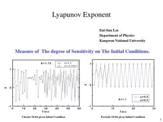
Sensitive dependence on the initial conditions • Definition: A set S exhibits sensitive dependence ifr>0 s.t. >0 and xS y s.t |x-y|< and |xn-yn|>r for some n. The sensitive dependence of the trajectory on the initial conditions is a key element of deterministic chaos! pendulum A: =-140°,d/dt=0pendulum B: =-140°1',d/dt=0 Demonstration However…
Sensitivity on the initial conditions also happens in linear systems But this is “explosion process”, not the deterministic chaos! xn+1= 2xn Why? There is no boundness. • SIC leads to chaos only if the trajectories are bounded (the system cannot blow up to infinity). • With linear dynamics either SIC or bounded trajectories. With nonlinearities could be both. There is no folding without nonlinearities!
The Lyapunov Exponent • A quantitative measure of the sensitive dependence on the initial conditions is theLyapunov exponent . It is the averaged rate of divergence (or convergence) of two neighboring trajectories in the phase space. • Actually there is a whole spectrum of Lyapunov exponents. Their number is equal to the dimension of the phase space. If one speaks about the Lyapunov exponent, the largest one is meant.
Definition of Lyapunov Exponents • Given a continuous dynamical system in an n-dimensional phase space, we monitor the long-term evolution of an infinitesimal n-sphere of initial conditions. • The sphere will become an n-ellipsoid due to the locally deforming nature of the flow. • The i-th one-dimensional Lyapunov exponent is then defined as following: p1(t) p1(0) x(t) t - time flow x0 p2(0) p2(t)
On more formal level • The Multiplicative Ergodic Theorem of Oseledec states that this limit exists for almost all points x0 and almost all directions of infinitesimal displacement in the same basin of attraction.
Order: λ1> λ2 >…> λn • The linear extent of the ellipsoid grows as 2λ1t • The area defined by the first 2 principle axes grows as 2(λ1+λ2)t • The volume defined by the first 3 principle axes grows as 2(λ1+λ2+λ3)t and so on… • The sum of the first j exponents is defined by the long-term exponential growth rate of a j-volume element.
Signs of the Lyapunov exponents • Any continuous time-dependent DS without a fixed point will have 1 zero exponents. • The sum of the Lyapunov exponents must be negative in dissipative DS at least one negative Lyapunov exponent. • A positive Lyapunov exponent reflects a “direction” of stretching and folding and therefore determines chaos in the system.
The signs of the Lyapunov exponents provide a qualitative picture of a system’s dynamics • 1D maps: ! λ1=λ: • λ=0 – a marginally stable orbit; • λ<0 – a periodic orbit or a fixed point; • λ>0 – chaos. • 3D continuous dissipative DS: (λ1,λ2,λ3) • (+,0,-) – a strange attractor; • (0,0,-) – a two-torus; • (0,-,-) – a limit cycle; • (-,-,-) – a fixed point.
The sign of the Lyapunov Exponent • <0-the system attracts to a fixed point or stable periodic orbit. These systems are non conservative (dissipative) and exhibit asymptoticstability. • =0-the system is neutrally stable. Such systems are conservative and in a steady state mode. They exhibit Lyapunov stability. • <0-the system is chaotic and unstable. Nearby points will diverge irrespective of how close they are.
Computation of Lyapunov Exponents • Obtaining the Lyapunov exponents from a system with known differential equations is no real problem and was dealt with by Wolf. • In most real world situations we do not know the differential equations and so we must calculate the exponents from a time series of experimental data. Extracting exponents from a time series is a complex problem and requires care in its application and the interpretation of its results.
Calculation of Lyapunov spectra from ODE (Wolf et al.) • A “fiducial” trajectory (the center of the sphere) is defined by the action of nonlinear equations of motions on some initial condition. • Trajectories of points on the surface of the sphere are defined by the action of linearized equations on points infinitesimally separated from the fiducial trajectory. • Thus the principle axis are defined by the evolution via linearized equations of an initially orthonormal vector frame {e1,e2,…,en} attached to the fiducial trajectory
Problems in implementing: • Principal axis diverge in magnitude. • In a chaotic system each vector tends to fall along the local direction of most rapid growth. (Due to the finite precision of computer calculations, the collapse toward a common direction causes the tangent space orientation of all axis vectors to become indistinguishable.) Solution: Gram-Schmidt reorthonormalization (GSR) procedure!
The linearized equations act on {e1,e2,…,en} to give a set {v1,v2,…,vn}. Obtain {v’1,v’2,…,v’n}. Reorthonormalization is required when the magnitude or the orientation divergences exceeds computer limitation. GSR:
GSR never affects the direction of the first vector, so v1 tends to seek out the direction in tangent space which is most rapidly growing, |v1|~ 2λ1t; • v2 has its component along v1 removed and then is normalized, so v2 is not free to seek for direction, however… • {v’1,v’2} span the same 2D subspace as {v1,v2}, thus this space continually seeks out the 2D subspace that is most rapidly growing|S(v1,v2)|~2(λ1+λ2)t … |S(v1,v2…,vk)|~2(λ1+λ2+…+λk)t k-volume • Somonitoring k-volume growth we can find first k Lyapunov exponents.
Example for Henon map An orthonormal frame of principal axis vectors {(0,1),(1,0)} is evolved by applying the product Jacobian to each vector:
Result of the procedure: • Consider: • J multiplies each current axis vector, which is the initial vector multiplied by all previous Js. • The magnitude of each current axis vector diverges and the angle between the two vectors goes to zero. • GSR corresponds to the replacement of each current axis vector. • Lyapunov exponents are computed from the growth of length of the 1-st vector and the area. 1=0.603; 2=-2.34
Lyapunov spectrum for experimental data(Wolf et al.) • Experimental data usually consist of discrete measurements of a single observable. • Need to reconstruct phase space with delay coordinates and to obtain from such a time series an attractor whose Lyapunov spectrum is identical to that of the original one.
Implementation Details • Selection of embedding dimension and delay time: emb.dim>2*dim. of the underlying attractor, delay must be checked in each case. • Evolution time between replacements: maximizing the propagation time, minimizing the length of the replacement vector, minimizing orientation error. • Henon attractor: the positive exponent is obtained within 5% with 128 points defining the attractor. • Lorenz attractor:the positive exponent is obtained within 3% with 8192 points defining the attractor.
Time Horizon • When the system has a positive , there is a time horizon beyond which prediction breaks down (even qualitative). • Suppose we measure the initial condition of an experimental system very accurately, but no measurement is perfect – let |0| be the error. • After time t: |(t)|~|0|et, if a is our tolerance, then our prediction becomes intolerable when |(t)|a and this occurs after a time
Demonstration |0| t=thorizon • No matter how hard we work to reduce measurement error, we cannot predict longer than a few multiples of 1/. Prediction fails out here t=0, 2 initial conditions almost indistinguishable |(t)|~|0|et
So, after a million fold improvement in the initial uncertainty, we can predict only 2.5 times longer! Example
Some philosophy • The notion of chaos seems to conflict with that attributed to Laplace: given precise knowledge of the initial conditions, it should be possible to predict the future of the universe. However, Laplace's dictum is certainly true for any deterministic system. • The main consequence of chaotic motion is that given imperfect knowledge, the predictability horizon in a deterministic system is much shorter than one might expect, due to the exponential growth of errors.