Download
1 / 38
380 likes | 593 Views
Eco 6351 Economics for Managers Chapter 11a. Aggregate Supply and Demand. Prof. Vera Adamchik. Jobs. Internal market forces. Prices. External shocks. Growth. Output. Policy levers. International balances. The macro economy. DETERMINANTS. OUTCOMES. MACRO ECONOMY. Macro view.

E N D
Eco 6351Economics for ManagersChapter 11a. Aggregate Supply and Demand Prof. Vera Adamchik
Jobs Internal market forces Prices External shocks Growth Output Policy levers International balances The macro economy DETERMINANTS OUTCOMES MACRO ECONOMY
Macro view The determinants of macro performance include: • Internal market forces — Population growth, spending behavior, invention and innovation, and the like. • External shocks — Wars, natural disasters, trade disruptions, and so on. • Policy levers — Tax policy, government spending changes in the availability of money, and regulation.
Potential GDP • The quantity of real GDP supplied when unemployment is at its natural rate and there is full employment is called potential real GDP. • Over the business cycle, employment fluctuates around full employment and real GDP fluctuates around potential GDP.
Two time horizons • To study the economy at full employment and over the business cycle, we distinguish two time frames: - the macroeconomic long run, - the macroeconomic short run.
The macroeconomic long runis a time frame that is sufficiently long for economic forces to bring real GDP to potential (full-employment) GDP. • The macroeconomic short run is a period during which real GDP has fallen below or risen above potential GDP. At the same time, the unemployment rate has risen above or fallen below the natural rate.
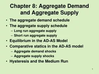
The Aggregate Supply-Aggregate Demand model The AS-AD model enables us to understand three features of macroeconomic performance: • Growth of potential GDP • Inflation • Business cycle fluctuations
Long-run aggregate supply • The long-run aggregate supply is vertical because potential GDP is independent of the price level. • A movement along the LRAS is accompanied by a change in two sets of prices: the prices of goods and services and the prices of productive resources. When relative prices remain constant, real GDP also remains constant.
PRICE LEVEL (average price) REAL OUTPUT (quantity per year) Long-run aggregate supply Long Run Aggregate Supply Potential (Full Employment) GDP
Aggregate demand Other things remaining the same, the higher the price level, the smaller is the quantity of real GDP demanded. This relationship between the quantity of real GDP demanded and the price level is called aggregate demand.
Aggregate demand • The AD curve is the relationship between the quantity of real GDPdemanded and the price level in a given time-period, ceteris paribus. • The AD curve is downward-sloping: the higher the price level, the smaller is the quantity of real GDP demanded. Reasons: real balances effect, foreign trade effect, interest rate effect.
PRICE LEVEL (average price) REAL OUTPUT (quantity per year) Aggregate demand Higher prices Lower prices Aggregate demand Less output demanded More output demanded
Stable or unstable • The central concern of macroeconomic theory is whether the internal forces of the marketplace will generate desired outcomes.
Classical theory • Prevalent theory prior to the 1930s. • The economy is stable because of its ability to self-adjust. • The cornerstones of the Classical Theory are flexible prices and flexible wages. • According to Classical economists, government intervention in a self-adjusting macroeconomy is unnecessary.
Say’s Law • According to Say’s Law, “supply creates its own demand.” • Unsold goods will ultimately be sold when buyers and sellers find an acceptable price. • In the labor market, some people will be unemployed, but can find new jobs if they are willing to accept lower wages.
The Great Depression • The Great Depression (1929-1939) was a stunning blow to Classical economists. • In the Depression’s worst year, 1933, the production of U.S. farms, factories, shops, and offices was only 70 percent of its 1929 level and 25 percent of the labor force was unemployed. • The science of economics had no solutions to the Great Depression.
24 20 16 12 8 ANNUAL RATE OF INFLATION OR UNEMPLOYMENT (percent) 4 0 – 4 – 8 1900 1910 1920 1930 1940 Inflation and Unemployment, 1900 – 1940 Unemployment Prices
The Keynesian revolution • John Maynard Keynes provided an alternative to the Classical Theory. • In 1936, Keynes published The General Theory of Employment, Interest, and Money.
Keynes asserted that the private economy was inherently unstable. No self-adjustment. • In Keynes’ view, the inherent instability of the marketplace required government intervention (“Policy levers”).
Keynes focused primarily on the short term. He wanted to cure an immediate problem almost regardless of the long-term consequences of the cure. “In the long run,” said Keynes, “we’re all dead.” • Keynes believed that after his cure for depression had restored the economy to a normal condition, the long-term problems of inflation and slow economic growth will return.
Short-run aggregate supply The short-run aggregate supply curve is the relationship between the quantity of real GDPsupplied and the price level in a given time-period, ceteris paribus. That is, when the money wage rate and other resource prices remain constant.
Short-run aggregate supply • The aggregate supply curve is upward-sloping: the output increases when price level rises. • The aggregate supply curve is relatively flat when capacity is underutilized. It begins to slope upward as producers approach capacity.
Shape of the SRAS curve • Short-Run Aggregate Supply (SRAS) has three segments or ranges: • Horizontal range (Keynesian segment), • Intermediate (Upward-sloping) range, • Vertical range (Classical segment)
Short-run aggregate supply P Vertical range Price level Horizontal range Upward-sloping or intermediate range Q Real domestic output, GDP
Macroeconomic equilibrium • Macroeconomic equilibrium occurs when the quantity of real GDP demanded equals the quantity of real GDP supplied.
Macro-equilibrium: Real output and the price level P SRAS Equilibrium in the Horizontal Range Price Level Pe AD Q Q1 Qe Q2 Real Domestic Output, GDP
Macro-equilibrium: Real output and the price level P SRAS Equilibrium in the Intermediate Range Price Level Pe P1 AD Q Q1 Qe Q2 Real Domestic Output, GDP
Macro failure • There are two potential problems with macro equilibrium — undesirability and instability.
Macro Failure • Undesirability — the price-output relationship at equilibrium may not satisfy our macroeconomic goals • Undesirable Outcomes: • Unemployment • Recession • Inflation
Three types of short-run macroeconomic equilibrium (1) below full-employment equilibrium (real GDP is less than potential GDP and there is a recessionary gap); (2) above full-employment equilibrium (real GDP exceeds potential GDP and there is an inflationary gap); (3) at full-employment equilibrium (real GDP equals potential GDP).
PRICE LEVEL (average price) REAL OUTPUT (quantity per year) Below FE equilibrium Aggregate demand Aggregate supply E PE F P* Equilibrium output Full employment QE QF
Macro failure • Instability — even if designated macro equilibrium is optimal, it may be displaced by macro disturbances. • Shifts in aggregate supply and aggregate demand can upset a full employment equilibrium.
Recurrent shifts • Business cycles are a result of recurrent shifts of the aggregate supply and demand curves. • There are lots of reasons to expect aggregate supply and aggregate to shift.
PRICE LEVEL (average price) PRICE LEVEL (average price) REAL OUTPUT (quantity per year) REAL OUTPUT (quantity per year) Macro disturbances (a) Supply shifts (b) Demand shifts AS1 AS0 AS0 AD0 G F P1 F P* P* H P2 AD0 AD1 Q1 QF Q2 QF
PRICE LEVEL (average price) REAL OUTPUT (quantity per year) Origins of a recession:Demand shifts AS0 E0 E1 AD0 AD1 Q1 QF
PRICE LEVEL (average price) REAL OUTPUT (quantity per year) Origins of a recession:Supply shifts AS1 AS0 E2 E0 AD0 Q2 QF
PRICE LEVEL (average price) REAL OUTPUT (quantity per year) Origins of a recession:Supply and demand shift AS1 AS0 E3 E0 AD0 AD1 Q3 QF