What is MPC?
What is MPC?. Hypothesis testing. Is the MPC 0.8?. Typically we tell intro macro students that MPC is 0.8 Our OLS estimate is 0.756 Does this mean that 0.8 is wrong? In this sample: yes! But in the population: not clear. Statistical Inference. Same issue as with gender example

What is MPC?
E N D
Presentation Transcript
What is MPC? Hypothesis testing
Is the MPC 0.8? • Typically we tell intro macro students that MPC is 0.8 • Our OLS estimate is 0.756 • Does this mean that 0.8 is wrong? • In this sample: yes! • But in the population: not clear
Statistical Inference • Same issue as with gender example • We may have a weird (slightly) sample that by pure chance gives us 0.756 when the true value is 0.8 • We want a formal procedure that will answer the question: • Is the difference between 0.756 and 0.8 large enough to enable use to reject the idea that the true MPC is 0.8?
OLS Estimates are RV • The first step in a formal procedure is to note that the OLS estimators are themselves random variables. • The precise value of the estimate depends on precise sample • Since sample choice is random so is the precise value of the estimate • If we observed the entire population there would be no distribution
OLS Estimator is RV • The key issue is that both are functions of the data so the precise value of each estimate will depend on the particular data points included in the sample which is random • This observation is the basis • statistical inference • and all judgments regarding the quality of estimates (see later).
OLS as RV Sounds Weird? • How can a random estimate be any use? • The estimate is not entirely random • It will be close to the true value on average (more later) • But deviation from truth is random
OLS as RV • To illustrate the impact of the sample on estimates, try different samples • Split the sample into 100 mini samples and run regression • Different samples will produce different “b” • The file distribution.do does this for you • Plot histogram of answers • Is it “normal”? • In reality we don’t calculate the distribution using this method.
OLS is Normal • Usually assume the estimators have a normal distribution • How can we say this? • OLS estimators are linear functions of the data so if the data has a normal distribution then so will the OLS estimators • This makes use of one of the properties of Normal distributions that we reviewed • The data will have a normal distribution if the residual has a normal distribution • True because model is linear: Yi = 1+2Xi+ui • Use The CLT (more later) whichapplies to large samples
Why Normality? • The assumption of normality is made for convenience • Easier to work with predefined distribution than histograms • Is it reasonable? • We had our doubts previously • Example: share prices • Econometricians must be honest with themselves
Distribution of bOLS • “Sampling distribution of the estimator” • OLS is unbiased so the distribution is cantered on the true value • Its variance depends on the variance of the residuals • Estimate produced by stata • bOLS is normally distributed
Hypothesis Testing • Non-trivial because of sampling distribution • Is the evidence consistent with the null hypothesis being true? • “Null hypothesis” is our preconceived notion • General approach • what would the distribution look like if the (null) hypothesis was true? • Where on the distribution is our estimate? • How likely is our estimate to occur when the hypothesis is true? • How likely is the hypothesis to be true?
A Criminal Trial • Metaphor of a criminal trial • We have the hypothesis that the accused is innocent • We ask if the evidence is consistent with the hypothesis being true • If not we can reject the hypothesis • If yes we fail to reject • Note: don’t “accept” the hypothesis
Mechanism for Hypothesis Test • State the Hypothesis we want to test H0: bMPC= 0.8 H1: bMPC≠ 0.8 • Calculate the distribution of bOLS assuming that H0 is true. • Stata provides the stn. error of b • Locate our estimate on the distribution • What is the probability that our estimate would have come from this distribution? • Does this lead us to believe the null hypothesis?
Any estimate is possibly consistent with any hypothesis • Always the possibility of a real fluke even with no mistakes • But some are clearly more likely than others • We can measure the probability of an estimate occurring if we know the distribution of the estimator • Clearly it is possible to get an estimate of 0.756 if the true value is 0.8
What is the probability? • P(bOLS<0.756| bMPC=0.8)=? • P(z <(0.756-0.8)/0.0307205)) • P(z< -1.43226836 )= 0.07603 • So there is an 8% chance that our estimate (or lower) would have arisen in a world where the true value is 0.8 • How do we interpret this?
So what is the answer? • What does this say about the likelihood of 0.8 being the true value? • Free to make your own judgement • 8% seems a little low • but 5% is the usual threshold • some times 10% or 1% is the threshold • So we cannot use this data to reject the idea that true value is 0.8 • “Cannot reject the Null Hypothesis”
So what is the answer? • If we use 10% as our threshold then we can reject the hypothesis • Be sure you understand the differences between the two answers • The criminal trial metaphor may help • Now days it has become usual for researchers to report the probability
Another Example Use the individual consumption data • State the Hypothesis we want to test H0: bMPC= 0.6 H1: bMPC≠ 0.6 • Calculate the distribution of bOLS assuming that H0 is true. • Find our estimate on the distribution • What is the probability that our estimate would have come from this distribution? • Does this lead us to believe the null hypothesis?
Again any estimate could be consistent with this hypothesis • What is the probability of a fluke now? • Clearly fairly unlikely to get an estimate of 0.756 if the true value is 0.6 • Probability is much less than 5% • P(bOLS>0.756| bMPC=0.6)=0.00001 • So we “can reject” the hypothesis • i.e. We can use this data to reject the notion that the true value is 0.6 • Same result for any threshold unless ridiculously small
Some Comments • Criminal Trial metaphor: The null hypothesis (innocence) will only be overturned if there is overwhelming evidence • What constitutes “overwhelming” • Not with regard to the size of the difference between values forb(compare the two examples). • it is the difference in probability • i.e. the distance on the distribution
What Have We Learned? • OLS estimates the line of best fit • This line can be interpreted as the conditional expectation • OLS estimators are random variables so we need to do statistical inference • What matters is not absolute the difference between estimated and hypothesised values but the probability of that difference
What is Missing? • We have only one X variable • Our hypothesis test procedure is a little cumbersome • We have only dealt with hypotheses that relate to one coefficient being equal to some number