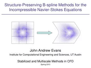
Structure-Preserving B- spline Methods for the Incompressible Navier -Stokes Equations

Structure-Preserving B-spline Methods for the Incompressible Navier-Stokes Equations John Andrew Evans Institute for Computational Engineering and Sciences, UT Austin Stabilized and MultiscaleMethods in CFD Spring 2013

Motivation • So why do we need another flow solver? • Incompressibility endows the Navier-Stokes equations with importantphysical structure: • Mass balance • Momentum balance • Energy balance • Enstrophy balance • Helicity balance • However, most methods only satisfy theincompressibility constraint in an approximate sense. • Such methods do not preserve structure and lack robustness.

Motivation Consider a two-dimensional Taylor-Green vortex. The vortex is a smooth steady state solution of the Euler equations.

Motivation Conservative methods which only weakly satisfy incompressibility do not preserve this steady state and blow up in the absence of artificial numerical dissipation. 2-D Conservative Taylor-Hood Element Q2/Q1 and h = 1/8

Motivation Methods which exactly satisfy incompressibility are stable in the Euler limit and robust with respect to Reynold’s number. Increasing Reynold’s number 2-D Conservative Structure-preserving B-splines k’= 1 and h = 1/8

Motivation • Due to the preceding discussion, we seek new discretizations that: • Satisfy the divergence-free constraint exactly. • Harbor local stability and approximation properties. • Possess spectral-like stability and approximation properties. • Extend to geometrically complex domains. Structure-Preserving B-splines seem to fit the bill.

The Stokes Complex The classical L2 de Rham complex is as follows: From the above complex, we can derive the following smoothedcomplex with the same cohomology structure:

Scalar Potentials Vector Potentials Flow Pressures Flow Velocities The Stokes Complex The smoothed complex corresponds to viscous flow, so we henceforth refer to it as the Stokescomplex.

The Stokes Complex • For simply-connected domains with connected boundary, the Stokes complex is exact. • grad operator maps onto space of curl-freefunctions • curl operator maps onto space of div-free functions • div operator maps onto entire space of flow pressures

The Stokes Complex Gradient Theorem: Curl Theorem: Divergence Theorem:

Discrete Flow Velocities Discrete Flow Pressures Discrete Scalar Potentials Discrete Vector Potentials The Discrete Stokes Subcomplex • Now, suppose we have a discrete Stokes subcomplex. • Then aGalerkindiscretizationutilizing the subcomplex: • Does not have spurious pressure modes, and • Returns a divergence-free velocity field.

The Discrete Stokes Subcomplex

Ξ = {0, 0, 0, 0.2, 0.4, 0.6, 0.8, 0.8, 1, 1, 1}, k = 2 Knots w/ multiplicity Start w/ piecewise constants Bootstrap recursively to k Structure-Preserving B-splines Review of Univariate (1-D) B-splines: Knot vector on (0,1) and k-degree B-spline basis on (0,1) by recursion:

Structure-Preserving B-splines Review of Univariate (1-D) B-splines: • Open knot vectors: • Multiplicity of first and last knots is k+1 • Basis is interpolatory at these locations • Non-uniform knot spacing allowed • Continuity at interior knot a function of knot repetition k=2

Structure-Preserving B-splines Review of Univariate (1-D) B-splines: • Derivatives of B-splines are B-splines onto k=4 k=3

Structure-Preserving B-splines Review of Univariate (1-D) B-splines: • We form curves in physical space by taking weighted sums. 4 5 3 2 0 “control mesh” 1 - control points - knots Quadratic basis:

polynomial degree in direction i ith continuity vector Structure-Preserving B-splines Review of Multivariate B-splines: • Multivariate B-splines are built through tensor-products • Multivariate B-splines inherit all of the aforementioned properties of univariate B-splines In what follows, we denote the space of n-dimensional tensor-product B-splines as

Structure-Preserving B-splines Review of Multivariate B-splines: • We form surfaces and volumes using weighted sums of multivariate B-splines (or rational B-splines) as before. Mesh Control mesh

Structure-Preserving B-splines Two-dimensional Structure-Preserving B-splines Define for the unit square: In the context of fluid flow: and it is easily shown that:

Structure-Preserving B-splines Two-dimensional Structure-Preserving B-splines: Mapped Domains On mapped domains, the Piola transform is utilized to map flow velocities. Pressures are mapped using an integral preserving transform.

Structure-Preserving B-splines Two-dimensional Structure-Preserving B-splines We associate the degrees of freedom of structure-preserving B-splines with the control mesh. Notably, we associate:

Structure-Preserving B-splines Two-dimensional Structure-Preserving B-splines, k1 = k2 = 2:

Structure-Preserving B-splines Three-dimensional Structure-Preserving B-splines Define for the unit cube: It is easily shown that:

Structure-Preserving B-splines Three-dimensional Structure-Preserving B-splines Flow velocities: map w/ divergence-preserving transformation Flow pressures: map w/ integral-preserving transformationVector potentials: map w/ curl-conserving transformation

Structure-Preserving B-splines Three-dimensional Structure-Preserving B-splines We associate as before the degrees of freedom with the control mesh.

Structure-Preserving B-splines Three-dimensional Structure-Preserving B-splines Control points:Scalar potential DOF Control edges: Vector potential DOF

Structure-Preserving B-splines Weak Enforcement of No-Slip BCs • Nitsche’s method is utilized to weakly enforce the no-slip condition in our discretizations. Our motivation is three-fold: • Nitsche’s method is consistent and higher-order. • Nitsche’s method preserves symmetry and ellipticity. • Nitsche’s method is a consistent stabilization procedure. Furthermore, with weak no-slip boundary conditions, a conforming discretization of the Euler equations is obtained in the limit of vanishing viscosity.

Structure-Preserving B-splines Weak Enforcement of Tangential Continuity Between Patches On multi-patch geometries, tangential continuity is enforced weakly between patches using a combination of the symmetric interior penalty method and upwinding.

Summary of Theoretical Results Steady Navier-Stokes Flow • Well-posedness for small data • Optimal velocity error estimates and suboptimal, by one order, pressure error estimates • Conforming discretization of Euler flow obtained in limit of vanishing viscosity (via weak BCs) • Robustness with respect to viscosity for small data

Summary of Theoretical Results Unsteady Navier-Stokes Flow • Existence and uniqueness (well-posedness) • Optimal velocity error estimates in terms of the L2 norm for domains satisfying an elliptic regularity condition (local-in-time) • Convergence to suitable weak solutions for periodic domains • Balance laws for momentum, energy, enstrophy, and helicity • Balance law for angular momentum on cylindrical domains

Spectrum Analysis Spectrum Analysis Consider the two-dimensional periodic Stokes eigenproblem: We compare the discrete spectrum for a specified discretization with the exact spectrum. This analysis sheds light on a given discretization’s resolution properties.

Spectrum Analysis Spectrum Analysis: Structure-Preserving B-splines

Spectrum Analysis Spectrum Analysis: Taylor-Hood Elements

Spectrum Analysis Spectrum Analysis: MAC Scheme

Selected Numerical Results Steady Navier-Stokes Flow:Numerical Confirmation of Convergence Rates 2-D Manufactured Vortex Solution

Selected Numerical Results Steady Navier-Stokes Flow:Numerical Confirmation of Convergence Rates Robustness with respect to Reynolds number k’= 1 and h = 1/16 2-D Manufactured Vortex Solution

Selected Numerical Results Steady Navier-Stokes Flow:Numerical Confirmation of Convergence Rates Instability of 2-D Taylor-Hood with respect to Reynolds number Q2/Q1 and h = 1/16 2-D Manufactured Vortex Solution

U H H Selected Numerical Results Steady Navier-Stokes Flow:Lid-Driven Cavity Flow

Selected Numerical Results Steady Navier-Stokes Flow:Lid-Driven Cavity Flow at Re = 1000

Structure-Preserving B- spline Methods for the Incompressible Navier -Stokes Equations