Download
1 / 75
750 likes | 986 Views
Empirical Models Based on the Universal Soil Loss Equation Fail to Predict Discharges from Chesapeake Bay Catchments. Boomer, Kathleen B. Weller, Donald E. Jordan, Thomas E. of the Smithsonian Environmental Research Center. Journal of Environmental Quality, 2008. Presentation Overview.

E N D
Empirical Models Based on the Universal Soil Loss Equation Fail to Predict Discharges from Chesapeake Bay Catchments Boomer, Kathleen B. Weller, Donald E. Jordan, Thomas E. of the Smithsonian Environmental Research Center Journal of Environmental Quality, 2008
Presentation Overview • Abstract • Background Information • Methods • Location • Water Quality Data • Spatial Data • Data Analysis • Results/Discussion • Conclusion • My Comments • Open Discussion
1. Abstract Goal: Accurately predict sediment loads/yields in un-gauged basins. Methods:Test the most widely used equation, USLE with accurate water quality data significant number of catchments from 2 different agencies. Also attempt a multiple linear regression approach. Results:The USLE and all its derivatives perform very poorly, even using SDR’s. So does the multiple linear regression. Conclusion:USLE & multiple linear regression are not advised.
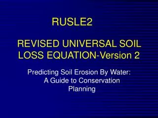
2. Background Information The Universal Soil Loss Equation A = R K LS CP A = estimated long-term annual soil loss (Mg soil loss ha−1 yr−1) R = rainfall and runoff factor representing the summed erosive potential of all rainfall events in a year (MJ mm ha−1 h−1 yr−1) L = slope length (dimensionless) S = slope steepness (dimensionless) K = soil erodibility factor representing units of soil loss per unit of rainfall erosivity (Mg ha h ha−1 MJ−1 mm−1) CP = characterizes land cover and conservation management practices (dimensionless).
2. Background Information The Revised Universal Soil Loss Equation 2 incorporate a broader set of land cover classes and attempt to capture deposition in complex terrains More sub-factors Daily time step
2. Background Information Universal Soil Loss Equation = Edge of Field
2. Background Information Universal Soil Loss Equation = Catchment Scale
2. Background Information Sediment Delivery Ratios
2. Background Information Sediment Delivery Ratios 1. Estimate from calibration data or 2. Use complex spatial algorithms Yagow 1998 SEDMOD Transport Exported from Field Observed at WQ site
2. Background Information Models that rely on USLE for calibration GWLF (Generalized Watershed Loading Function; Haith and Shoemaker, 1987) AGNPS (AGricultural Non-Point Source; Young et al., 1989) SWAT (Soil & Water Assessment Tool; Arnold and Allen, 1992) HSPF (Hydrological Simulation Program-Fortran; Bicknell et al., 1993) SEDD (Sediment Delivery Distributed model; Ferro and Porto, 2000).
2. Background Information DANGER!!! GROSS EROSION VS. SEDIMENT TRANSPORT FIELD OBSERVATIONS VS. REGIONAL SPATIAL DATA Van Rompaey et al., 2003 – 98 catchments in europe, poor results Wischmeier and Smith 1978; Risse et al., 1993; Kinnell, 2004a) – Not for Catchment
3. Methods Water Quality Data
3. Methods Water Quality Data SERC DATA continuous monitoring stations in 78 basins within 166,000 km2 Chesapeake Bay watershed 5-91,126 ha across physiographic regions Coastal Plain = 45 Piedmont = 10 Mesozoic Lowland = 7 Appalachian Mountain = 9 Appalachian Plateau = 7 selected across a range of land cover proportions no reservoirs, no point sources
0-40% 0-82% 0-39% 2-100% 3. Methods Water Quality Data SERC DATA
3. Methods Water Quality Data USGSS DATA continuous monitoring stations in 23 additional basins within 166,000 km2 Chesapeake Bay watershed 101-90,530 ha no reservoirs
0-30% 0-40% 5-100% 3. Methods Water Quality Data USGS DATA
3. Methods Water Quality Data SERC WATER QUALITY DATA • Automated samplers, continuous stage, • flow-weighted water samples composited weekly • <= 1 year, 1974-2004 • Annual mean flow rates * flow-weighted mean conc = annual avg loads • Yield=load/area USGS WATER QUALITY DATA • Samples collected daily or determined by ESTIMATOR model
3. Methods Regional Spatial Data
3. Methods Regional Spatial Data USLE Analysis
3. Methods USLE Analysis GRID-BASED USLE ANALYSIS RKLSCP RKLSCP RKLSCP R (rainfall erosivity) = Derivded from linear interpolation of national iso-erodent map RKLSCP RKLSCP RKLSCP RKLSCP RKLSCP RKLSCP
3. Methods USLE Analysis GRID-BASED USLE ANALYSIS RKLSCP RKLSCP RKLSCP K(surface soil erodibility)= STATSGO resampled to 30m RKLSCP RKLSCP RKLSCP RKLSCP RKLSCP RKLSCP
3. Methods USLE Analysis GRID-BASED USLE ANALYSIS RKLSCP RKLSCP RKLSCP L (slope length) = NED DEM resampled to 30 m RKLSCP RKLSCP RKLSCP RKLSCP RKLSCP RKLSCP
3. Methods USLE Analysis GRID-BASED USLE ANALYSIS RKLSCP RKLSCP RKLSCP S(slope steepness)= NED DEM resampled to 30 m RKLSCP RKLSCP RKLSCP RKLSCP RKLSCP RKLSCP
3. Methods USLE Analysis GRID-BASED USLE ANALYSIS RKLSCP RKLSCP RKLSCP C(cover management)= Consolidated NLCD 30m RKLSCP RKLSCP RKLSCP RKLSCP RKLSCP RKLSCP ***no differentiation of erosion control practices
3. Methods USLE Analysis GRID-BASED USLE ANALYSIS RKLSCP RKLSCP RKLSCP P (support practice factor) = 1 RKLSCP RKLSCP RKLSCP RKLSCP RKLSCP RKLSCP ***no differentiation of erosion control practices
3. Methods Revised-USLE2 Analysis
3. Methods RUSLE-2 • Automated • identifies potential sediment transport routes using raster grid cumulation and max downhill slope methods • Identifies depositional zones • L= surface overland flow distance from origin to deposition or stream • CP (cover and practice) calculated from the RUSLE database (wider range of land cover characteristics)
3. Methods SDR’s
3. Methods SDR’s 3 LUMPED-PARAMETER 2 SPATIALLY EXPLICIT “where life is a box and space is only considered in terms of area” “life is a box, but spatial relationships matter”
3. Methods Runoff
3. Methods Runoff (for multiple linear regression) CN (curve number) method used to estimate runoff potential and annual runoff STATSGO hydrosoilgrp + LC = CN Monthly time step annual value
3. Methods Multiple Linear Regression
3. Methods Multiple Linear Regression • Considered additional parameters • Physiographic province • Watershed size • Variation in terrain complexity • Topographic relief ratio • Land cover proportions • Percent impervious area • Runoff potential • Annual average runoff (CN method)
4. Results USLE vs RUSLE2
4. Results USLE vs RUSLE 2
4. Results USLE vs RUSLE 2 USGS Data Pearson r = 0.95, p<0.001
4. Results USLE & RUSLE2 (SDR) vs SERC & USGS
4. Results USLE & RUSLE2 (SDR) vs SERC & USGS
4. Results USLE & RUSLE2 (SDR) vs SERC & USGS Negative spearmen r =
4. Results USLE & RUSLE2 (SDR) vs SERC & USGS Negative spearmen r = All p values = not statistically significant
4. Results USLE Parameters vs USLE
4. Results USLE parameters vs USLE
4. Results Univariate Regressions
4. Results Univariate Regressions