GG313 Lecture 24 11/17/05 Power Spectrum, Phase Spectrum, and Aliasing
220 likes | 404 Views
GG313 Lecture 24 11/17/05 Power Spectrum, Phase Spectrum, and Aliasing.

GG313 Lecture 24 11/17/05 Power Spectrum, Phase Spectrum, and Aliasing
E N D
Presentation Transcript
GG313 Lecture 24 11/17/05 Power Spectrum, Phase Spectrum, and Aliasing
The primary display used in the frequency display is commonly called the Power Spectrum. It is a plot that shows a measure of the power in each frequency interval, where power is defined as the square of the amplitude. Power is calculated from the Fourier coefficients. Recall: (5.102) The Power in y at frequency j is just Ak2=aj2+ bj2. Thus we can generate a plot of power vs. frequency by plotting Ak2 vs frequency. While this plot is strictly a “periodogram”, most people call it a power spectrum. A “real” power spectrum is defined as the Fourier transform of the autocorrelation function.
Examples of power spectra: Fig.5. Seismic noise spectra from the borehole seismometers at JT-1. Z and H1,H2 denote the noise spectra estimated from the vertical component and the horizontal components respectively. HNM and LHN indicate typical noise spectra from the land observatories. The noise spectra at JT-1 show that JT-1 can provide good quality data. NOISE SPECTRA FROM A BOREHOLE SEISMOMETER IN THE NW PACIFIC OCEAN.
Time Domain Bottle-nose dolphin sound Frequency Domain
This is a sample of the Radio Spectrum. Each peak is the location of a broadcast station. The frequency is in MegaHz.
Spectrograms Each vertical line is a power spectrum. Colors represent different power.
We can also think of the power spectrum as yielding which frequencies contribute most to the variance of the signal. The larger the amplitude, the higher the variance. In fact, the variance is shown to be: (5.109) In practice, the periodogram is not a very stable plot - small changes in the signal can lead to large changes in individual spectral estimates (Aj). To get around this, we often average several spectral estimates together to smooth the spectrum or we average several spectra to reduce the variance of each spectral estimate. More about this when we discuss filters.
While the power spectrum and spectrogram (for non-stationary time series) are probably the most common forms of display in the frequency domain, one can also plot the phase spectrum, where the phase angle is given by: (5.104) The phase spectrum is important when determining the effect of a filter on a time series - to be discussed later.
One critical aspect of spectral analysis occurs when a critical assumption is violated. This assumption is that all energy occurs at frequencies below the Nyquist frequency. When this is not the case, ALIASING occurs. Aliasing can be a “feature” or a big problem. The critical fact is that energy at frequencies above the Nyquist doesn’t disappear, it gets shifted to frequencies below the nyquist. The demonstration below illustrates several points: the connection of spectral analysis to music (middle-C is 261.63 Hz), what an “octave” is, how good your ear is at spectral analysis (which implies strongly that spectral analysis is important for your survival), and the effects of aliasing.
Aliasing Demo http://ptolemy.eecs.berkeley.edu/eecs20/week13/aliasing.html Middle-C is 261.63 Hz 523 1046 2093 4186 60 Hz Can you detect any distortion?
Wessel wagon wheel aliasing: http://www.soest.hawaii.edu/pwessel/courses/gg313/wheel.html It’s easy to see from the figure above that aliasing moves high frequencies to lower frequencies because samples are not taken often enough. Can we predict what frequency the aliased energy will show up at?
At the nyquist frequency (Nyq=1/2t) there are two samples per cycle. This is just enough to get an accurate representation. At twice the nyquist (2 Nyq=1/ t , the sampling frequency), there is one sample per cycle, and the resulting signal has zero frequency. At 3Nyq, we’re back up to the Nyquist again.
Can you think of any reason why you might want to alias a signal? In radio, you might want to take a signal and move it up to the frequency of the station, and then re-sample it at a much lower frequency in the receiver after radio transmission to recover the original signal.
In most cases, aliasing is BAD. Your desired signal is corrupted with energy aliased from frequencies beyond the Nyquist, and, once there, you cannot get rid of it. How can you prevent aliasing? • sample at a high enough frequency to cover all energy or • filter your data before sampling so that it contains only energy below the nyquist. Such a filter is known as an anti-aliasing filter.
The continuous spectrum The periodogram gives estimates of the energy at discrete frequencies, but it is just an estimate based on some sample of the population. If we took many samples we would find that the uncerrtainty of the spectral estimates was equal to about the estimate itself. There are two ways to reduce this uncertainty: Increase the length of the time series. This leads to more spectral estimates within the same Nyquist, so you can average adjacent estimates to improve the variance. Average the spectral estimates from several samples of equal length and T.
Transform pairs: When going from the time domain to the frequency domain and back there are several transform pairs that are worth remembering. These are specific time domain signals that have characteristic frequency domain transforms. Each provides insight to a property of the transformation. The transformations work both ways, and which side is the time domain and which is the frequency domain is not important. Notice in these transforms how the spacing changes from one domain to the other - a “t” in one domain becomes a “1/t” in the other.
This representation in the frequency domain is somewhat different than what we’ve used before. Now we have NEGATIVE FREQUENCIES. A negative frequency is easy to interpret - it’s a rotation (like the wagon wheel) that goes in the opposite direction of the true motion. Right now,it’s a convenience for presenting some characteristics of the transforms. DELTA FUNCTION: A delta function in this case is a single non-zero point in a long line of zeroes. Note that it’s transform has equal energy in all frequencies. EXERCISE: Generate a 64-point time series of zeroes, with a 1 at point 32. Take its fft. What do you get? Change the 1 to a 2. How does this change the fft? How do the values of the spectral estimates relate to the size of the delta function?
Using Matlab’s fft function, you get complex values for the spectral estimates. To change them to power spectral estimates multiply each estimate by its complex conjugate: P=Y.*conj(Y), where y=fft(data) and then plot P. What happens if you move the impulse to any other point? Nothing changes? How about the phase spectrum? You can get the phase response by doing phase=angle(Y); Try plotting that with the impulse in different locations.
BOXCAR: Use the same 64-point zeros function, but replace points 5-9 with ones. { y(5:9)=[1 1 1 1 1] } and calculate the power spectrum. Does it look like the boxcar transform I showed? Why not? How does the maximum power relate to the size of the boxcar? Would this power spectrum change if the number of points was increased to 128? What would happen if all values were 1? Then you would only get the DC (zero frequency) term. What if only one value were 1 ?
This shows the reciprocity of the transform. It doesn’t matter which is the time domain or which is the frequency domain. Note with the boxcar that the first zero crossing occurs at a frequency of 1/d where d is the width of the boxcar.