Download
1 / 43
430 likes | 535 Views
Analysis of Algorithms. Maximum weight matching. Uri Zwick May 2014. TexPoint fonts used in EMF. Read the TexPoint manual before you delete this box.: A A A A A. Maximum Weight Matching. Find a matching whose total weight is maximal. 3. 22. 6. 8. 15. 4. 18. 1. 5. 25. 2.

E N D
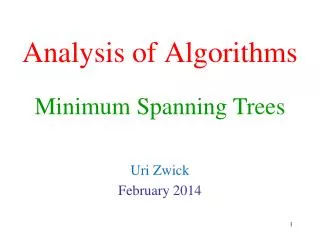
Analysis of Algorithms Maximum weight matching Uri Zwick May 2014 TexPoint fonts used in EMF. Read the TexPoint manual before you delete this box.: AAAAA
MaximumWeight Matching Find a matching whose total weight is maximal 3 22 6 8 15 4 18 1 5 25 2 Maximum weight matching
MaximumWeight Matching Find a matching whose total weight is maximal 3 22 6 8 15 4 18 1 5 25 2 An augmenting path that increases the size of the matching, but not the total weight of the matching
MaximumWeight Matching The maximum matching problem in bipartite graphs can be easily reduced to a min cost flow problem The bipartite case, also known as the assignment problem, can be solved in O(mn+n2log n) time [Kuhn (1955)] The problem in non-bipartite graphs is harder. First polynomial time algorithm given by [Edmonds (1965)] An O(mn+n2log n)-time implementation of Edmonds’ algorithm was given by [Gabow (1990)] An O(mn1/2log(nN))-time algorithm for the non-bipartite case, where all weights are integers of absolute value at most N, given by [Gabow-Tarjan (1991)] An O(m−1log−1)-time (1−)-approximation algorithm for the non-bipartite case given recently by [Duan-Pettie (2014)]
Alternating paths and cycles with respect to a given matching M The weightwM(P) of an alternating path/cycle Pw.r.t. M is the sum of the weights of the edges not in M, minus the sum of the weights of the edges in M + + − + − + − − + + − Lemma: If P is a proper alternating path or cycle, i.e., an alternating path such that its endpoints are either unmatched, or matched by the edges touching them in P, then MP is also a matching and w(MP)=w(M)+wM(P)
Improving paths or cycles Theorem: M is a matching of maximum weight iff there are no proper alternating paths or cycles of positive weight w.r.t. M If P is a proper alternating path or cycle with wM(P) > 0, thenw(MP) = w(M)+wM(P) > w(M) If w(M’) > w(M),thenat least one alternating path or cycle in MM’ must have positive weight
Maximum weight augmenting paths Theorem: Let M be a matching of maximum weight among all matchingsof size |M|, let Pbe an augmenting path w.r.t. Mof maximum weight wM(P). Then, MP is of maximum weight among all matchingsof size |M| + 1. Let M’ bea matching of maximum weight among all matchings of size|M| + 1. If P is an augmenting path w.r.t. M then wM(P) ≤ w(M’) −w(M) If P is an augmenting path w.r.t. M in MM’, then wM(P) = w(M’) −w(M).Otherwise M’P contradicts the choice of M,as w(M’P) = w(M’)−wM(P) > w(M). MM’ contains at least one augmenting path w.r.t. M
The assignment problem The maximum weight matching problem in bipartitegraphs is also known as the assignment problem Possible application: Assigning people to tasks.Each person can only perform a single task.Each task can only be performed by a single person. The “Hungarian method” [Kuhn (1955)] [Jacobi (1865)?] Efficient implementation in O(mn+n2logn) time We shall derive it in two different ways
Algorithm for the assignment problem Start with M0 = .(A maximum weight matching with no edges) In each iteration, find a maximum weight augmenting path Piw.r.t. Mi and let Mi+1Mi Pi(Miis a maximum weight matching containing iedges) Return the maximum weight matching found Can stop when the weight of Piis non-positive(To be justified later) How do we find maximum weight augmenting paths? In bipartite graphs, can be reduced to computing a shortest path
Finding maximum weight augmenting paths in bipartite graphs G = (U ,V ,E) Direct unmatched edges from U to V Direct matched edges from V to U Add a source s and a sink tConnect them to unmatched vertices Negate the weights of the edges not in the matching Find a shortest path from s to t V U Such a shortest path is a maximum weight augmenting path
Finding maximum weight augmenting paths in bipartite graphs G = (U ,V ,E) Since M is a maximum weight matching of size |M|, there are no negative cycles Can use Bellman-Ford to finda shortest path in O(mn) time Yields an O(mn2)-time algorithm Slow! V U We show how to use Dijkstraand reduce time to O(mn+n2logn)
Linear Programming formulationof the assignment problem Is this really a valid formulation? Who says that (P) has an integral solution?
Linear Programming formulationof the assignment problem Three different ways of showing that the formulation is valid: 1) Direct proof. If x is an optimal solution, we convert it into an integral solution without decreasing its value 2) The matrix A in the LP formulation, which is just the incidence matrix of the graph, is totally unimodular, i.e., the determinant of every square submatrix is 1,0 or +1. 3) Our algorithm will always find an integral optimal solution
Direct proof Let xe be an optimal solution and assume that some of the values are fractional We show that the number of fractional values can be reduced without decreasing the value xewe of the soluion There is either a path of fractional edges between two unsaturated vertices, or an even cycle of fractional edges Alternatingly, add and subtract from the xevalueson the path or cycle + − + can be positive or negative xewe does not change! Choose so that at least one fractional xebecomes 0 or 1
Incidence matrix of a (bipartite) graph Edges e u 1 U Vertices v 1 V Every column contains exactly two 1s The incidence matrix of a bipartite graph is totally unimodular,i.e., the determinant of every square submatrix is 1,0 or +1.
The primal-dual method(a.k.a the “Hungarian method”) Keep :1) an integral feasible primal solution, i.e., a matching M2) A dual feasible solution y Maintain the first set of complementary slackness conditions:(u,v)M yu + yv = wu,v Our goal is to satisfy the second set of complementary slackness conditions:yu> 0 u matched In each iteration we either augment M, or adjust y sothat more complementary slackness conditions are satisfied
The Primal-dual methodPreliminaries Start with:
The Primal-dual method G=(U,V,E) Grow an alternating forest fromall unmatched vertices of Uusing only tight edges Let S be the vertices of U in the forest, and T be the vertices of V in the forest If an augmenting path is found, augment M What do we do if we are “stuck”? (The forest cannot be extended, using tight edges, and the dual variables of some unmatched vertices are still positive)
Adjustingthe dual variables All edges leaving the forest, from even vertices, are nottight Slack of edges connecting two vertices in the forest is unchanged All forest edges and matched edges are still tight Slack of edges leaving the forest from even vertices decreases by If =1, then yu=0 for every root u and we are done! If =2, we have at least one new tight edge
Adjustingthe dual variables All edges leaving the forest, from even vertices, are nottight Thus, 1 is the joint yvalue of the roots
Linear Programming formulation of the generalweighted matching problem [Edmonds (1965)] Enough to have |B| odd (P) has an exponential number of constraints (D) has an exponential number of variables
Linear Programming formulation of the generalweighted matching problem [Edmonds (1965)] Correctness of formulation would follow from algorithm B with zB> 0 are blossoms Note the similarity of dual with odd vertex cover
The Primal-dual methodThe non-bipartite case Primal solution: A matching M Dual values yv≥ 0, for vVA collection of (nested) blossomsA dual value zB≥ 0 for each blossom B Dual solution: Ablossom Bw.r.t. M is full, i.e., it contains (|B|−1)/2 edges of M
The Primal-dual methodThe non-bipartite case Primal solution: A matching M Dual values yv≥ 0, for vVA collection of (nested) blossomsA dual value zB≥ 0 for each blossom B Dual solution: Complementary slackness conditions: Always maintain (1) and (3)Make progress towards (2)
Correctness If the algorithm terminates, correctness follows from weak duality Or directly: Let M be the matching found and M’ an arbitrary matching
More fun with blossoms In the cardinality case, after each augmentation we expanded all blossoms and started from scratch We cannot do that here, as blossoms now have dual values Lemma: A blossom remains a blossom after an augmentation, possibly with no stem. We thus start each phase with a collection of blossoms During a phase, new blossoms may be formed, and existing blossoms may be expanded In the cardinality case, blossoms were always even Blossoms may now be added as odd vertices
The alternating forest All vertices are blossoms(some nested some trivial) All edges in the forest are tight All edges in blossoms are tight,even if they are not in the forest When there are no more tightedges to explore, adjust dual variables
The Primal-dual methodInitialization Start with:
Adjusting the dual variables All edges leaving the forest, from even vertices, are nottight
Case 1: = 1 After the update, yv=0, for every v unmatched All complementary slackness conditions are satisfied We are done! • Case 2: = 2 After the update, at least one more edge leaving the forest from an even vertex is tight We can extend the forest while keeping all invariants
Case 3: = 3 An edge connecting two even vertices in different blossoms becomes tight If the blossoms are in different trees augmenting path Otherwise, a new even blossom B is formedSet zB 0 The new even blossom swallows some odd blossomsAll vertices in these blossoms become even andtight edges leaving them may be explored
Case 4: = 4 zBbecomes 0, for some oddblossomB, Expand the odd blossom B Neweven blossom B Theseblossoms leave the forest
Number of steps Does the algorithm terminate? The algorithm is composed of at most n/2 phases in which an augmenting path is found After each adjustment of the dual variables, either we are done, or an augmenting path is found, or the number of even vertices increases Thus, in each phase there are at most nadjustments of the dual variables Total number of dual adjustment steps is O(n2) Algorithm is polynomial! [Edmonds (1965)]
Number of steps After each adjustment of the dual variables, either we are done, or an augmenting path is found, or the number of even vertices increases Case 1: We are done Case 2: The forest is extended. The new odd blossom added is either unmatched (an augmenting path found), or an even blossom is immediately added Case 3: Either an augmenting path is found or a new blossom is formed. The new blossom swallows some odd vertices that are now even Case 4: An odd blossom is expanded. Some of its vertices become even
Efficient implementation Maintaining blossoms and finding augmenting paths Similar to the unweighted case, though now we also have to expand blossoms Maintaining slacks and computing Completely naïve implementation of each step in O(m) time, giving an O(mn2)-time algorithm Using some (sophisticated) data structures we can implement each phase in: O(n2) [Gabow(1976)] [Lawler (1976)] O(m logn) [Galil-Micali-Gabow(1986)] O(m +n logn) [Gabow(1990)]