Assessing Diurnal SST Variability in Coupled Ocean-Atmosphere Models: A Methodological Approach
This document outlines the management activities related to the ECMWF Summer Seminars held in September 2011, focusing on coupled data assimilation tasks involving Sea Surface Temperature (SST) analyses. Key participants, Chris Old and Orial Kryeziu, have initiated a project to evaluate discrepancies between satellite observations and model outputs. The objective is to identify areas for improving coupled modeling systems. Deliverables include assessment reports, documentation of visualization software, and strategies for evaluating SST-related inconsistencies to enhance model performance.

Assessing Diurnal SST Variability in Coupled Ocean-Atmosphere Models: A Methodological Approach
E N D
Presentation Transcript
ECMWF Summer Seminars September 2011
Task 3: Management Activities • OrialKryeziu recruited started June 18th • September coupled DA workshop • Chris Old recruited starting 1st October • Weekly Skype meetings Reading and Edinburgh started 1st October • Outline • Chris Old: Background on SST in Reanalyses and Observations • OrialKryeziu: Progress on extending SST matchups • Chris Old: Uncertainty in SST products for Coupled Data Assimilation
Task 3: Deliverables • KO+ 9 months D6 (initial): A current reanalysis assessment report identifying case study periods and showing areas where coupled model improvements may be expected • KO+15 months D7: Documentation for Opensource Visualisation software and demonstrator presenting comparisons between ocean and atmosphere reanalysis products using the observation operator codes developed for assimilation, and observations, particularly near ocean surface, for scientific and outreach use • KO+24 months D6 (final): An final impact assessment report based on Task 1, WP3.3 and 3.4 studies, describing improved representations of coupled phenomena and improved fitting to observational data.
Satellite SST in Coupled Data Assimilation Chris Old and Chris Merchant School of GeoSciences, The University of Edinburgh ESA Data Assimilation Projects, Progress Meeting 1 11th December 2012, The University of Reading
Satellite SST in Coupled Data Assimilation ObsERVATIONvs Model Inconsistencies
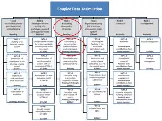
Satellite SST in coupled data assimilation Task 3: Evaluating observation strategies The key objective of this task is to review the correlated variability of surface oceanic and atmospheric datasets, both within the coupled model systems and with the observations themselves. These results will provide input to the development of a set of test experiments (Task 4), by identifying suitable test periods and data sets. WP3.1 Consistency of current surface ocean and atmospheric analysis products Use satellite measurements as a baseline to examine any inconsistencies within the products, e.g. regions where there are discrepancies in SSTs between atmosphere and ocean products, such as regions where strong (or weak) SST diurnal cycles are detected but where the analysed surface wind speeds seem too high (or low). Introduction
Observed SST Diurnal Variability Solar heating produces near surface thermal stratification, while wind driven mixing erodes diurnal stratification. Modification of instantaneous air-sea heat flux from warm-layer formation can be 50 Wm-2. Amplitude of cycle often observed up to 4K, larger events are observed (>6K). dSST excursions spatially and temporally coherent. dSST event magnitude and horizontal length scale anti-correlated. Extreme dSST maxima arise where low wind speed sustained from early morning to mid-afternoon. Observed dSST between 9AM and 2PM on 2nd June 2006. Data from the SEVIRI instrument on MSG2. References:Gentemann et al., 2008; Merchant et al., 2008 Introduction
Methodology First stage in the process is to look for instances of discrepancy between observed and simulated diurnal SSTs. Use SST data retrieved from SEVIRI on MSG2 to calculate observed diurnal SST. Simulate diurnal SST using a statistical model based on ERA wind and heat flux fields. Use the difference between observed and simulated dSST to identify regions of inconsistency between model fields and observations. Apply this test to a long time series of model fields and observations to determine current state of modelling capability. Use the results to identify a set of suitable data periods that can be used test the performance of the new coupled assimilation systems being developed. Introduction
Statistical Model for dSST Diurnal SST difference for a time t after start of warming Integrated heat flux during warming period Maximum 10m wind speed during warming period Coefficient functions ( LUTs ) Constructed using ERA40 reanalysis atmosphere data and SST retrieved from SEVIRI data. Reference: Filipiak et al., 2012 Methodology
Application to ALADIN DW database Calculate observed dSSTobs between 9am and 2pm (local solar time) Exclude pixels with in 0.2° of land (land surface temperature contamination) Exclude pixels where SDI > 0.5 at any point during the day (dust contamination) Exclude pixels where dSSTobs < -1.4K (cloud contamination) Calculate dSSTsim using statistical model (based on NWP reanalysis fields) Calculate Δ(dSST) = dSSTobs- dSSTsim Locate peak values where |Δ(dSST)| > 1.5K (threshold of significant difference) Locate all pixels around peak where |Δ(dSST)| > 1.0K (identify coherent regions) Eliminate regions that are too small (fewer than 40 points) Δ(dSST) > 1.5K modelled wind fields too large Δ(dSST) < -1.5K modelled wind fields too weak Methodology
Example of method – 2nd June 2006 SEVIRI Statistical Model (ERA Interim Fields) Methodology
Observed - Modelled dSST – 2nd June 2006 Case 1: Wind speed too large Observed – Modelled dSST difference ( K ) Case 2: Wind speed too low Case3: Wind field offset Methodology
Inconsistent regions – 2nd June 2006 Methodology
ERA 40 compared with ERA Interim Using ERA40 data Using ERA Interim data Methodology
Sea Surface Diurnal Warming OrialKryeziu, Keith Haines Diurnal Warming: sub-daily variations in sea surface temperature (SST) defined relative to the temperature prior to diurnal stratification (foundation temperature). Achievements: Implemented diurnal warming observation operator codes for ERA40, ERAInterim and ALADIN and compared with SEVIRI data Extended search area to include full SEVERI disk data (June 2006), data obtained Apr 2006 – Sept 2008 Obtained ERAInterim 3 hourly wind data based on interleaved forecasts, to test sensitivity of diurnal SST Observation operator code Initiated dialogue with ECMWF on incorporating surface wave data into diurnal model
- The SST data are hourly observations from SEVIRI spanning -100°W to 45°E and -60°S to 60°N mapped on a 0.05° resolution grid. Currently, data is available for one month: June 2006. Also available from SEVIRI is the “Saharan dust index” (SDI)- non-dimensional index based on infra-red wavelengths. - Peak-to-peak mean amplitude in dSST for the ocean as whole is 0.25 K. Largest dSSTs exceed 6K, and affect 0.01% of the surface (Filipiak et al., 2012).
Winds fields (ERA-interim, 3 hourly) derived from a numerical prediction model (NWF) are obtained from ECMWF. The winds in the western Mediterranean and European Seas are heavily defined by land-sea contrasts and orographic effects. Diurnal warming cases occur frequently in this region.The picture shows the mean of the reciprocal of the wind speed between 0900 and 1500 h UTC.
Mean maximum value of dSST here shows correlation with the mean reciprocal of the wind strength. It is useful to consider knowledge of frequent local wind fields to see orographic influences on diurnal variability. For example:- Surface winds accelerated through the Corsica and Sardinia passage (Merchant et al. 2008).- Mistral winds are often responsible for the clear, sunny weather in the Golfe du Lion. Mistral Wind
Extreme cases (>4K) arise under conditions with persistent light winds and strong sunlight. Sustained low winds in the morning are rare. In the North and Baltic Seas a prevalent factor in diurnal warming is the optical attenuation coefficient of water (Merchant et al. 2008).
There is an anti-correlation between the magnitude and the length scale of dSST events. Also the scales of areas of sustained low winds are smaller than those of instantaneously low winds. A few examples of dSST>4 (14pm - 9am):18th of June 2006
Conclusions: Extreme diurnal events (peak dSST > 4K) are observed by SEVIRI. In the Mediterranean sea orographic influence is an important factor. In the North and Baltic Seas, optical attenuation coefficient of water is a (significant ) driving factor. Sustained low winds are required for extreme warming events to be observed. Future work: 1) Extend Case criteria to using other near-surface variables: Sea state information: Wave data from ERAInterim; Scatterometerand Altimetricsatellite data 2) Develop uncertainty model for SST L2 coupled reanalysis.
Satellite SST in Coupled Data Assimilation SSTobs Error Covariances
Uncertainties for SST assimilation WP3.1 Consistency of current surface ocean and atmospheric analysis products The space-time sampling of satellite data will be assessed against spatial and temporal variability of the ocean and atmospheric reanalysis fields. This sampling uncertainty will be used in combination with uncertainty components from other sources developed in the ARC SST and SST CCI projects. Coupled Data Assimilation Workshop : An understanding and quantification of satellite SST error covariance length scales in time and space can be used to constrain the coupled assimilation of surface fields. Little work has been done to date to quantify satellite based SST error covariance length scales. Observation Error Covariance
Components of SST uncertainty • Radiometric noise • Usually random (but variable) • 1/√n averaging over n pixels • Algorithmic • Geographically systematic component • Variable component usually correlated to synoptic scales ( average ≠ 1/√n ) • Sampling • Spatial sub-sampling (only clear sky) - representativity • Time within diurnal cycle of SST • Outliers • cloud, aerosol problems Observation Error Covariance
Radiometric noise • Noise equivalent differential temperature (NEdT) • NEdT = SD of errors in brightness temperatures • Propagates simply to SST random uncertainty • Can depend on • Variations in coefficients • Channel set • Scene temperature • Instrument properties and state • Time (degradation) • Random uncertainty in SST varies in calculable way between SSTs Observation Error Covariance
Algorithmic Errors Algorithmic limitations in coping with varying atmospheric conditions. Synoptically correlated in time and space. Error distributions can be simulated. BTs, y Least squares regression + Radiative Transfer SSTs, x Coefficients, a Observation Error Covariance
Instantaneous simulation of retrieval error Observation Error Covariance
Instantaneous simulation of retrieval error Observation Error Covariance
Instantaneous simulation of retrieval error Observation Error Covariance
Instantaneous simulation of retrieval error Observation Error Covariance
Instantaneous simulation of retrieval error Observation Error Covariance
Instantaneous simulation of retrieval error Observation Error Covariance
Instantaneous simulation of retrieval error Observation Error Covariance
Temporal correlation scales r ~ ( 1/e time scale ) / days Observation Error Covariance
Spatial correlation scales Zonal Meridional Approximation to r ~ ( 1/e length scales ) / km Observation Error Covariance
Error Covariance Work Plan • Proposed approach: • Choice of case study: new AATSR L2P* ( full resolution product ) • Simulate retrieval error fields • Calculate covariance information • Re-grid onto an assimilation grid ( ECMWF input required ) • Can also flag “trusted, independent obs” set for model testing • * Currently being developed at CEMS under NCEO and contains ARC/SST CCI uncertainty information Observation Error Covariance
References: Gentemann, C. L., P. J. Minnett, P. Le Borgne, C. J. Merchant. 2008. Multi-satellite measurements of large diurnal warming events. Geophysical Research Letter, 35, L22602 Merchant, C. J., M. J. Filipiak, P. Le Borgne, H. Roquet, E. Autret, J. -F. Piollé, S. Lavender. 2008. Diurnal warm-layer events in the western Mediterranean and European shelf. Geophysical Research Letter, 35, L04601 Filipiak, M. J., C. J. Merchant, H. Kettle, P. Le Borgne. 2012. An empirical model for the statistics of sea surface diurnal warming. Ocean Science, 8, 197-209