Download
1 / 16
160 likes | 260 Views
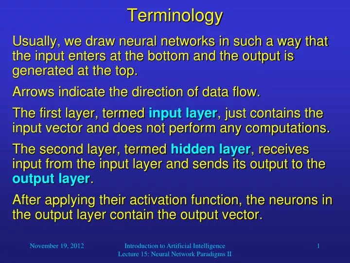
Terminology. Usually, we draw neural networks in such a way that the input enters at the bottom and the output is generated at the top. Arrows indicate the direction of data flow. The first layer, termed input layer , just contains the input vector and does not perform any computations.

E N D
Terminology • Usually, we draw neural networks in such a way that the input enters at the bottom and the output is generated at the top. • Arrows indicate the direction of data flow. • The first layer, termed input layer, just contains the input vector and does not perform any computations. • The second layer, termed hidden layer, receives input from the input layer and sends its output to the output layer. • After applying their activation function, the neurons in the output layer contain the output vector. Introduction to Artificial Intelligence Lecture 15: Neural Network Paradigms II
Terminology output vector • Example: Network function f: R3 {0, 1}2 output layer hidden layer input layer input vector Introduction to Artificial Intelligence Lecture 15: Neural Network Paradigms II
Linear Neurons • Obviously, the fact that threshold units can only output the values 0 and 1 restricts their applicability to certain problems. • We can overcome this limitation by eliminating the threshold and simply turning fi into the identity function so that we get: With this kind of neuron, we can build networks with m input neurons and n output neurons that compute a function f: Rm Rn. Introduction to Artificial Intelligence Lecture 15: Neural Network Paradigms II
Linear Neurons • Linear neurons are quite popular and useful for applications such as interpolation. • However, they have a serious limitation: Each neuron computes a linear function, and therefore the overall network function f: Rm Rn is also linear. • This means that if an input vector x results in an output vector y, then for any factor the input x will result in the output y. • Obviously, many interesting functions cannot be realized by networks of linear neurons. Introduction to Artificial Intelligence Lecture 15: Neural Network Paradigms II
fi(neti(t)) 1 0 neti(t) -1 1 Gaussian Neurons • Another type of neurons overcomes this problem by using a Gaussian activation function: Introduction to Artificial Intelligence Lecture 15: Neural Network Paradigms II
Gaussian Neurons • Gaussian neurons are able to realize non-linear functions. • Therefore, networks of Gaussian units are in principle unrestricted with regard to the functions that they can realize. • The drawback of Gaussian neurons is that we have to make sure that their net input does not exceed 1. • This adds some difficulty to the learning in Gaussian networks. Introduction to Artificial Intelligence Lecture 15: Neural Network Paradigms II
Sigmoidal Neurons • Sigmoidal neurons accept any vectors of real numbers as input, and they output a real number between 0 and 1. • Sigmoidal neurons are the most common type of artificial neuron, especially in learning networks. • A network of sigmoidal units with m input neurons and n output neurons realizes a network function f: Rm (0,1)n Introduction to Artificial Intelligence Lecture 15: Neural Network Paradigms II
fi(neti(t)) = 0.1 1 = 1 0 neti(t) -1 1 Sigmoidal Neurons • The parameter controls the slope of the sigmoid function, while the parameter controls the horizontal offset of the function in a way similar to the threshold neurons. Introduction to Artificial Intelligence Lecture 15: Neural Network Paradigms II
Supervised Learning in ANNs • In supervised learning, we train an ANN with a set of vector pairs, so-called exemplars. • Each pair (x, y) consists of an input vector x and a corresponding output vector y. • Whenever the network receives input x, we would like it to provide output y. • The exemplars thus describe the function that we want to “teach” our network. • Besides learning the exemplars, we would like our network to generalize, that is, give plausible output for inputs that the network had not been trained with. Introduction to Artificial Intelligence Lecture 15: Neural Network Paradigms II
Supervised Learning in ANNs • There is a tradeoff between a network’s ability to precisely learn the given exemplars and its ability to generalize (i.e., inter- and extrapolate). • This problem is similar to fitting a function to a given set of data points. • Let us assume that you want to find a fitting function f:RR for a set of three data points. • You try to do this with polynomials of degree one (a straight line), two, and nine. Introduction to Artificial Intelligence Lecture 15: Neural Network Paradigms II
deg. 2 f(x) deg. 1 deg. 9 x Supervised Learning in ANNs • Obviously, the polynomial of degree 2 provides the most plausible fit. Introduction to Artificial Intelligence Lecture 15: Neural Network Paradigms II
Supervised Learning in ANNs • The same principle applies to ANNs: • If an ANN has too few neurons, it may not have enough degrees of freedom to precisely approximate the desired function. • If an ANN has too many neurons, it will learn the exemplars perfectly, but its additional degrees of freedom may cause it to show implausible behavior for untrained inputs; it then presents poor ability of generalization. • Unfortunately, there are no known equations that could tell you the optimal size of your network for a given application; you always have to experiment. Introduction to Artificial Intelligence Lecture 15: Neural Network Paradigms II
The Backpropagation Network • The backpropagation network (BPN) is the most popular type of ANN for applications such as classification or function approximation. • Like other networks using supervised learning, the BPN is not biologically plausible. • The structure of the network is identical to the one we discussed before: • Three (sometimes more) layers of neurons, • Only feedforward processing: input layer hidden layer output layer, • Sigmoid activation functions Introduction to Artificial Intelligence Lecture 15: Neural Network Paradigms II
output vector y f(neto) … O1 OK … f(neth) H1 H2 H3 HJ … I1 I2 II input vector x The Backpropagation Network • BPN units and activation functions: Introduction to Artificial Intelligence Lecture 15: Neural Network Paradigms II
Learning in the BPN • Before the learning process starts, all weights (synapses) in the network are initialized with pseudorandom numbers. • We also have to provide a set of training patterns (exemplars). They can be described as a set of ordered vector pairs {(x1, y1), (x2, y2), …, (xP, yP)}. • Then we can start the backpropagation learning algorithm. • This algorithm iteratively minimizes the network’s error by finding the gradient of the error surface in weight-space and adjusting the weights in the opposite direction (gradient-descent technique). Introduction to Artificial Intelligence Lecture 15: Neural Network Paradigms II
f(x) slope: f’(x0) x0 x1 = x0 - f’(x0) x Learning in the BPN • Gradient-descent example: Finding the absolute minimum of a one-dimensional error function f(x): Repeat this iteratively until for some xi, f’(xi) is sufficiently close to 0. Introduction to Artificial Intelligence Lecture 15: Neural Network Paradigms II