Data Mining: Associations
Learn about frequent itemsets and association rules in data mining using the A-priori algorithm and its hash-based enhancements to analyze market baskets. Explore high-correlation mining and practical applications, such as detecting plagiarism and organizing web content.

Data Mining: Associations
E N D
Presentation Transcript
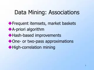
Data Mining: Associations • Frequent itemsets, market baskets • A-priori algorithm • Hash-based improvements • One- or two-pass approximations • High-correlation mining
Purpose • If people tend to buy A and B together, then a buyer of A is a good target for an advertisement for B. • The same technology has other uses, such as detecting plagiarism and organizing the Web.
The Market-Basket Model • A large set of items, e.g., things sold in a supermarket. • A large set of baskets, each of which is a small set of the items, e.g., the things one customer buys on one day.
Support • Simplest question: find sets of items that appear “frequently” in the baskets. • Support for itemset I = the number of baskets containing all items in I. • Given a support threshold s, sets of items that appear in >= s baskets are called frequent itemsets.
Example • Items={milk, coke, pepsi, beer, juice}. • Support = 3 baskets. B1 = {m, c, b} B2 = {m, p, j} B3 = {m, b} B4 = {c, j} B5 = {m, p, b} B6 = {m, c, b, j} B7 = {c, b, j} B8 = {b, c} • Frequent itemsets: {m}, {c}, {b}, {j}, {m, b}, {c, b}, {j, c}.
Applications 1 • Real market baskets: chain stores keep terabytes of information about what customers buy together. • Tells how typical customers navigate stores, lets them position tempting items. • Suggests tie-in “tricks,” e.g., run sale on hamburger and raise the price of ketchup. • High support needed, or no $$’s .
Applications 2 • “Baskets” = documents; “items” = words in those documents. • Lets us find words that appear together unusually frequently, i.e., linked concepts. • “Baskets” = sentences, “items” = documents containing those sentences. • Items that appear together too often could represent plagiarism.
Applications 3 • “Baskets” = Web pages; “items” = linked pages. • Pairs of pages with many common references may be about the same topic. • “Baskets” = Web pages p ; “items” = pages that link to p . • Pages with many of the same links may be mirrors or about the same topic.
Scale of Problem • WalMart sells 100,000 items and can store hundreds of millions of baskets. • The Web has 100,000,000 words and several billion pages.
Association Rules • If-then rules about the contents of baskets. • {i1, i2,…, ik} -> j • Means: “if a basket contains all of i1,…,ik, then it is likely to contain j. • Confidence of this association rule is the probability of j given i1,…,ik.
Example + _ _ + B1 = {m, c, b} B2 = {m, p, j} B3 = {m, b} B4 = {c, j} B5 = {m, p, b} B6 = {m, c, b, j} B7 = {c, b, j} B8 = {b, c} • An association rule: {m, b} -> c. • Confidence = 2/4 = 50%.
Finding Association Rules • A typical question is “find all association rules with support >= s and confidence >= c.” • The hard part is finding the high-support itemsets. • Once you have those, checking the confidence of association rules involving those sets is relatively easy.
Computation Model • Typically, data is kept in a “flat file” rather than a database system. • Stored on disk. • Stored basket-by-basket. • Expand baskets into pairs, triples, etc. as you read baskets. • True cost = # of Disk I/O’s. • Count # of passes through the data.
Main-Memory Bottleneck • In many algorithms to find frequent itemsets we need to worry about how main-memory is used. • As we read baskets, we need to count something, e.g., occurrences of pairs. • The number of different things we can count is limited by main memory. • Swapping counts in/out is a disaster.
Finding Frequent Pairs • The hardest problem often turns out to be finding the frequent pairs. • We’ll concentrate on how to do that, then discuss extensions to finding frequent triples, etc.
Naïve Algorithm • A simple way to find frequent pairs is: • Read file once, counting in main memory the occurrences of each pair. • Expand each basket of n items into its n(n-1)/2 pairs. • Fails if #items-squared exceeds main memory.
A-Priori Algorithm 1 • A two-pass approach called a-priori limits the need for main memory. • Key idea: monotonicity : if a set of items appears at least s times, so does every subset. • Converse for pairs: if item i does not appear in s baskets, then no pair including i can appear in s baskets.
A-Priori Algorithm 2 • Pass 1: Read baskets and count in main memory the occurrences of each item. • Requires only memory proportional to #items. • Pass 2: Read baskets again and count in main memory only those pairs both of which were found in Pass 1 to have occurred at least s times. • Requires memory proportional to square of frequent items only.
Picture of A-Priori Item counts Frequent items Counts of candidate pairs Pass 1 Pass 2
PCY Algorithm 1 • Hash-based improvement to A-Priori. • During Pass 1 of A-priori, most memory is idle. • Use that memory to keep counts of buckets into which pairs of items are hashed. • Just the count, not the pairs themselves. • Gives extra condition that candidate pairs must satisfy on Pass 2.
Picture of PCY Hash table Item counts Frequent items Bitmap Counts of candidate pairs Pass 1 Pass 2
PCY Algorithm 2 • PCY Pass 1: • Count items. • Hash each pair to a bucket and increment its count by 1. • PCY Pass 2: • Summarize buckets by a bitmap : 1 = frequent (count >= s ); 0 = not. • Count only those pairs that (a) are both frequent and (b) hash to a frequent bucket.
Multistage Algorithm • Key idea: After Pass 1 of PCY, rehash only those pairs that qualify for Pass 2 of PCY. • On middle pass, fewer pairs contribute to buckets, so fewer false drops --- buckets that have count s , yet no pair that hashes to that bucket has count s .
Multistage Picture First hash table Second hash table Item counts Freq. items Freq. items Bitmap 1 Bitmap 1 Bitmap 2 Counts of Candidate pairs
Finding Larger Itemsets • We may proceed beyond frequent pairs to find frequent triples, quadruples, . . . • Key a-priori idea: a set of items S can only be frequent if S - {a } is frequent for all a in S . • The k th pass through the file is counts the candidate sets of size k : those whose every immediate subset (subset of size k - 1) is frequent. • Cost is proportional to the maximum size of a frequent itemset.
Approximations All Frequent Itemsets At Most Two Passes
All Frequent Itemsets in <= 2 Passes • Simple algorithm. • SON (Savasere, Omiecinski, and Navathe). • Toivonen.
Simple Algorithm 1 • Take a main-memory-sized random sample of the market baskets. • Run a-priori or one of its improvements (for sets of all sizes, not just pairs) in main memory, so you don’t pay for disk I/O each time you increase the size of itemsets. • Be sure you leave enough space for counts.
Simple Algorithm 2 • Use as your support threshold a suitable, scaled-back number. • E.g., if your sample is 1/100 of the baskets, use s /100 as your support threshold instead of s . • Verify that your guesses are truly frequent in the entire data set by a second pass. • But you don’t catch sets frequent in the whole but not in the sample.
SON Algorithm 1 • Repeatedly read small subsets of the baskets into main memory and perform the simple algorithm on each subset. • An itemset becomes a candidate if it is found to be frequent in any one or more subsets of the baskets.
SON Algorithm 2 • On a second pass, count all the candidate itemsets and determine which are frequent in the entire set. • Key “monotonicity” idea: an itemset cannot be frequent in the entire set of baskets unless it is frequent in at least one subset.
Toivonen’s Algorithm 1 • Start as in the simple algorithm, but lower the threshold slightly for the sample. • Example: if the sample is 1% of the baskets, use 0.008s as the support threshold rather than 0.01s . • Goal is to avoid missing any itemset that is frequent in the full set of baskets.
Toivonen’s Algorithm 2 • Add to the itemsets that are frequent in the sample the negative border of these itemsets. • An itemset is in the negative border if it is not deemed frequent in the sample, but all its immediate subsets are. • Example: ABCD is in the negative border if and only if it is not frequent, but all of ABC , BCD , ACD , and ABD are.
Toivonen’s Algorithm 3 • In a second pass, count all candidate frequent itemsets from the first pass, and also count the negative border. • If no itemset from the negative border turns out to be frequent, then the candidates found to be frequent in the whole data are exactly the frequent itemsets.
Toivonen’s Algorithm 4 • What if we find something in the negative border is actually frequent? • We must start over again! • But by choosing the support threshold for the sample wisely, we can make the probability of failure low, while still keeping the number of itemsets checked on the second pass low enough for main-memory.
Low-Support, High-Correlation Finding rare, but very similar items
Assumptions 1. Number of items allows a small amount of main-memory/item. 2. Too many items to store anything in main-memory for each pair of items. 3. Too many baskets to store anything in main memory for each basket. 4. Data is very sparse: it is rare for an item to be in a basket.
Applications • While marketing may require high-support, or there’s no money to be made, mining customer behavior is often based on correlation, rather than support. • Example: Few customers buy Handel’s Watermusick, but of those who do, 20% buy Bach’s Brandenburg Concertos.
Matrix Representation • Columns = items. • Baskets = rows. • Entry (r , c ) = 1 if item c is in basket r ; = 0 if not. • Assume matrix is almost all 0’s.
In Matrix Form m c p b j {m,c,b} 1 1 0 1 0 {m,p,b} 1 0 1 1 0 {m,b} 1 0 0 1 0 {c,j} 0 1 0 0 1 {m,p,j} 1 0 1 0 1 {m,c,b,j} 1 1 0 1 1 {c,b,j} 0 1 0 1 1 {c,b} 0 1 0 1 0
Similarity of Columns • Think of a column as the set of rows in which it has 1. • The similarity of columns C1 and C2, sim (C1,C2), is the ratio of the sizes of the intersection and union of C1 and C2. (Jaccard measure) • Goal of finding correlated columns becomes finding similar columns.
Example C1 C2 0 1 1 0 1 1 sim (C1, C2) = 0 0 2/5 = 0.4 1 1 0 1
Signatures • Key idea: “hash” each column C to a small signature Sig (C), such that: 1. Sig (C) is small enough that we can fit a signature in main memory for each column. 2. Sim (C1, C2) is the same as the “similarity” of Sig (C1) and Sig (C2).
An Idea That Doesn’t Work • Pick 100 rows at random, and let the signature of column C be the 100 bits of C in those rows. • Because the matrix is sparse, many columns would have 00. . .0 as a signature, yet be very dissimilar because their 1’s are in different rows.
Four Types of Rows • Given columns C1 and C2, rows may be classified as: C1 C2 a 1 1 b 1 0 c 0 1 d 0 0 • Also, a = # rows of type a , etc. • Note Sim (C1, C2) = a /(a +b +c ).
Min Hashing • Imagine the rows permuted randomly. • Define “hash” function h (C ) = the number of the first (in the permuted order) row in which column C has 1.
Surprising Property • The probability (over all permutations of the rows) that h (C1) = h (C2) is the same as Sim (C1, C2). • Both are a /(a +b +c )! • Why? • Look down columns C1 and C2 until we see a 1. • If it’s a type a row, then h (C1) = h (C2). If a type b or c row, then not.
Min-Hash Signatures • Pick (say) 100 random permutations of the rows. • Let Sig (C) = the list of 100 row numbers that are the first rows with 1 in column C, for each permutation. • Similarity of signatures = fraction of permutations for which minhash values agree = (expected) similarity of columns.
Example C1 C2 C3 1 1 0 1 2 0 1 1 3 1 0 0 4 1 0 1 5 0 1 0 S1 S2 S3 Perm 1 = (12345) 1 2 1 Perm 2 = (54321) 4 5 4 Perm 3 = (34512) 3 5 4 Similarities: 1-2 1-3 2-3 Col.-Col. 0 0.5 0.25 Sig.-Sig. 0 0.67 0
Important Trick • Don’t actually permute the rows. • The number of passes would be prohibitive. • Rather, in one pass through the data: 1. Pick (say) 100 hash functions. 2. For each column and each hash function, keep a “slot” for that min-hash value. 3. For each row r , and for each column c with 1 in row r , and for each hash function h do: if h(r ) is a smaller value than slot(h ,c), replace that slot by h(r ).

