Download
1 / 1
10 likes | 117 Views
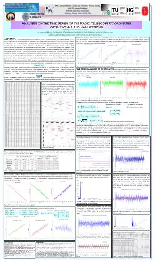
Analyses on the Time Series of the Radio Telescope Coordinates of the IVS-R1 and -R4 Sessions.

E N D
Analyses on the Time Series of the Radio Telescope Coordinates of the IVS-R1 and -R4 Sessions ABSTRACT:In this study, we investigate the coordinate time series of the radio telescopes which regularly take part for IVS-R1 and –R4 sessions. Firstly, we determine the deterministic parts of the series such as linear trend (velocity vectors of the antenna coordinates) due to e.g. crustal movements. Linear trends of the coordinate time series are estimated by least square (LS), fitting the coefficients of a linear regression function. After removing the linear trend from the series, sinusoidal (harmonic) variations of the series if they exist are determined by estimating the amplitude and phase of the Fourier series based on the frequency of the maximum spectral density (power) in the respective spectra plot (periodogram). To sample the data evenly linear interpolation is used. The spectral density of the data is produced by Fast Fourier Transform based on Discrete Fourier Transform. Most of the antennas harmonic variations are not found. Also, the amplitudes of the detected variations are small in ranges between 0.4 - 0.1 mm. This may be caused by the artifacts of the data interpolation or the data it self may not consist any harmonic variations. Because the geophysical models are already applied to the downloaded data (daily sinex normal equations of VLBI sessions provided by Deutsches Geodatisches Forschungsinstitut (DGFI)) except the models of atmosphere loading and thermal deformation. For further investigations of the coordinates to examine if they contain any sinusoidal variations after theremoval of the significant trends from seriesspectral analysis should be carried out. However, in Figure 5 from the time series of local topocentric coordinates of the site Svetloe, for year 2008 there is no significant trend in the up direction which means that directly cyclic variations should be investigated forthese kinds of series without removing the insignificant trend estimate. Figure 5. Time series of local topocentric coordinates of the site Svetloe The determination and removal of the offsets and linear trends (velocities) of coordinates is carried out by LS fit to the linear function. (1) where is the offsetwith respect to the mean coordinate value of the year, and is the trend and arethe residuals (Chatfield, 2004). The estimated parameters are divided by their standard deviations represent a statistics with degrees of freedom. If a parameter is to be judged as statistically different from zero, and thus significant, the computed t value (the test statistic) must be greater than,where is the level of confidence. Simply stated, the test statistic is (2) where is the standard deviation of the parameter. Table 1 shows the site velocities (trends) for the sites of which have adequate estimates (about 50 coordinate estimates per year) also for detecting annual and semi-annual tidal variations. TIME SERIES ANALYSIS OF COORDINATES:After reduction linear trend the resulted stationary series are analysed by means of detecting harmonics. This single spectral analysis approach known as auto spectral analysis based on the detection of the maximum power and respective frequency. The procedure is carried out iteratively eliminating the maximum amplitude up to reaching noise floor (Schuh, 1981). Figure 5. Kokee radio telescope coordinate series cleaned from trends In case a time series contains a periodic sinusoidal component with a known wavelength (frequency) the model will be :thesinusoidal variation: amplitude of the variation (6) : phase : stationary random series (7) (8) amplitude and phase of the variations of p th harmonics If we are interested in variation at low frequency of 1 cycle per year, then we should at least 1 year’s datain which case the lowest (fundamental) frequency we can fit is at 1 cycle per year. In other words, the lowest frequency covers the longest time period over the data. The lowest frequency depends on N which is the total number of the pairs of amplitudes of the harmonic analysis. The Nyquist frequency is the highest angular frequency () about which we can get meaningful information from a set of data. The Fourier series representation of the data is normally evaluated at the frequencies ( ) ofprovided from the fundamental ()frequency by multiplying the integers, called as Harmonics (Chatfield, 2004). In total, 17 radio telescope sites which have consistently taken part in most of the sessions from the beginning of 1994 to end of 2008 are included in our study. In Figure 1, the 17 VLBI sites that participated in the IVS-R1 and IVS-R4 24 hour (daily) sessions are shown. Figure 2 shows north, east and up components of the yearly site velocities and respective years are plotted. Figure 1. VLBI radio telescopes of IVS-R1 and R4 sessions Figure 2. Site velocities The coordinate time series of the VLBI antennas produced from the daily sinex normal equations of IVS-R1and -R4 sessions are unevenly spaced. As an example, sampling intervals are shown in Figure 6 for the antenna Wettzell. The mean of the sampling interval (e.g. antenna Wettzell up component 4 days) is used for producing the fundamental frequency (the maximum frequency data can produce). To form evenly spaced data linear interpolation (Trauth, 2007) is applied depending on the evenly-spaced (mean of the sampling interval) time axis (Figure 7). For the unevenly spaced data it seems to be impossible to prevent artifacts and spurious cycyles on the results to some extend since it is not possible to stay with in the range of the original data with any interpolation method.. E. Tanir(1), V. Tornatore(2), K. Teke(3,4) (1) Dept. of Geodesy and Photogrammetry Engineering, Karadeniz Technical University, Turkey (2) Dept. of Hydraulics, Environmental, Road Infrastracture, Remote Sensing Engineering, Politecnico di Milano, Italy (3) Institute of Geodesy and Geophysics, Vienna University of Technology, Austria (4) Dept. of Geodesy and Photogrammetry Engineering, Hacettepe University, Turkey Table 1. Velocities The velocities estimated in this study are almost equal to the ITRF 2005. Table 2 showsthe north, east and up components of the some antenna velocitiesof ITRF 2000 at epoch1997.0 . Table 2. Comparison between ITRF2000 and estimated velocity vectors Figure 6. sampling interval of the antenna Wettzell coordinate timeseries Figure 7. Resampling the data The Earth Centred Earth Fixed (ECEF) coordinates of the radio telescopes are estimated with minimumconstrained Least Squares adjustment from the daily sinex normal equations of VLBI sessions provided by Deutsches Geodatisches Forschungsinstitut (DGFI). The respective a priori station coordinates are computed from the coordinates of 25 globally distributed stations constrained to have NNR and NNT w.r.t. ITRF2000. Figure 3. Time series of the station coordinates ofAlgopark The power spectral density of the time series is computed by Fast Fourier Transform (Brigham, 1988) and ploted in Figure 8. The Fourier series (Eq.7) coefficients are estimated according to the period (360.8 days (fs = 0.00277) ) of maximum power with least squares. With the coefficients of the Fourier Series amplitude and phase of the maximum cyclic variation is provided (Eq.8). The amplitude and phase are found out 0.35 mm and -45.21°, respectively for the Wettzell up component. The Fourier series and the signal is shown in Figure 9. Figure 8. Autospectrum on the time series of the up component of the antenna Wettzell for the first iteration After the removal of the sinusoidal component from data (Figure 10) depending on the new period (360.8 days) the spectra of the residual is produced again (Figure 11). In every step harmonics are removed from the data based on the frequency of maximum power. The adjusted ECEF (ITRF2000) coordinates are transformed to the local topocentric coordinates as: estimation of respective covariances (4) (5) : longitude of station: latitude of station Figure 4. The time series of the local topocentric coordinates of the radio telescope WETTZEL Figure 9.The Fourier Series of the cyclic component that have the maximum power Figure 12. Spectra of first and last iteration for antenna Wetzell up component Figure 10.The remaining part of the time series - up component of the station Wettzell after eliminating the sinusoid of the first iteration • CONLUSIONS: • VLBI antenna coordinate velocities produced from IVS-R1 and –R4 sessions are approximately the same with the ITRF 2000 velocities of the same sites. • After removing the linear trend from the series, sinusoidal (harmonic) variations of the series (tidal variations of the antenna coordinates) if they exist are determined by estimating the amplitudes and phase of the Fourier series based on the frequency of the maximum spectral density (power) in the respective spectra plot (periodogram). • In most of the antennas harmonic variations are not found. • The amplitudes of the detected variations are small in ranges between 0.4 - 0.1 mm. This may be caused by the artifacts of the data interpolation carried out linearly or the data itself because of the un-modeled geophysical parts of the a priori coordinates derived. • The derived data daily sinex normal equations of VLBI sessions provided by DGFIhas already been modeled as a priori by certain geophysical models (e.g. troposphere, solid Earth tide, ocean loading, and pole tide) except atmosphere loading and thermal deformation. REFERENCES: Chatfield, C., 2004, The Analysis of Time Series An Introduction, Sixth Edition, Chapman & Hall/Crc, Washington, D.C, pp.121-146. Schuh, H., 1981, Zur Spektralanalyse von Erdrotationsschwankungen, sonderdruck aus: Die Arbeiten des Sonderforschungsbereiches 78 Satellitengeodäsie der Technichen Universität München im jahre 1980, Heft Nr. 41, München 1981, pp. 176-193. Trauth, H. Martin, 2007, MATLAB Recipes for Earth Sciences, 2nd Edition, Springer-Verlag Berlin Heidelberg, pp. 83-131. Wolf, R.P., and Ghilani, D.C., 1997, Adjustment Computations, John Wiley & Sons, Inc., pp.353-354, Newyork. Brigham, E. O., 1988, The fast Fourier transform and its applications, Prentice Hall Signal Processing Series. Englewood Cliffs. Figure 11.The significant sinusoids on the up component of Wettzell Table 3. Significant harmonics of the antenna coordinates