Download
1 / 49
590 likes | 877 Views
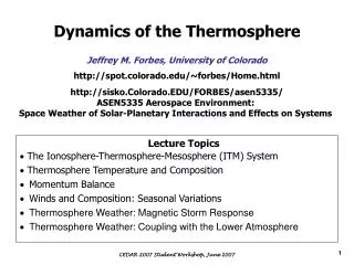
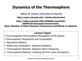
Dynamics of the Thermosphere. Jeffrey M. Forbes, University of Colorado http://spot.colorado.edu/~forbes/Home.html http://sisko.Colorado.EDU/FORBES/asen5335/ ASEN5335 Aerospace Environment: Space Weather of Solar-Planetary Interactions and Effects on Systems. Lecture Topics

E N D
Dynamics of the Thermosphere Jeffrey M. Forbes, University of Colorado http://spot.colorado.edu/~forbes/Home.html http://sisko.Colorado.EDU/FORBES/asen5335/ ASEN5335 Aerospace Environment: Space Weather of Solar-Planetary Interactions and Effects on Systems Lecture Topics • The Ionosphere-Thermosphere-Mesosphere (ITM) System • Thermosphere Temperature and Composition • Momentum Balance • Winds and Composition: Seasonal Variations • Thermosphere Weather: Magnetic Storm Response • Thermosphere Weather: Coupling with the Lower Atmosphere CEDAR 2007 Student Workshop, June 2007
The ITM System H Escape Magnetospheric Coupling B E B Energetic Particles 500 km Ion Outflow E Wind Dynamo Mass Transport Polar/Auroral Dynamics ITM System Joule Heating Wave Generation Solar Heating 60 km CO2 Cooling Turbulence NO Topographic Generation of Gravity Waves O3 Convective Generation of Gravity Waves & Tides CO2 CH4 solar-driven tides Planetary Waves H2O 0 km Pole Equator CEDAR 2007 Student Workshop, June 2007
Thermosphere Temperature & Composition CEDAR 2007 Student Workshop, June 2007
Temperature and Density Distributions and Ranges Diurnal and Solar Cycle CEDAR 2007 Student Workshop, June 2007
Atmospheric Composition CEDAR 2007 Student Workshop, June 2007
Momentum Balance CEDAR 2007 Student Workshop, June 2007
ion drag molecular viscosity (diffusion of momentum) pressure gradient Coriolis Substantial or convective derivative Thermodynamic Equation Continuity Equation Hydrostatic Law Equation of State Closed System for the Unknowns Horizontal Momentum Equation Governing Equations These equations are written in terms of total density & pressure; in practice, must actually consider multi-component equations, and self-consistent coupling between neutral species, and coupling with ionospheric and electrodynamic equations Momentum Equation CEDAR 2007 Student Workshop, June 2007
Coriolis force acts perpendicular to the wind vector. It deflects poleward winds towards the east and eastward winds equatorward. So, winds are driven clockwise (anticlockwise) in the northern (southern) hemisphere around pressure maxima. Near steady-state flow below about 150 km is usually involves approximate balance between the pressure gradient and Coriolis forces, leading to the geostrophic approximation, where the flow is parallel to the isobars (clockwise flow around a High in the Northern Hemisphere) Courtesy I. Mueller-Wodarg CEDAR 2007 Student Workshop, June 2007
The absence of any momentum sources at high levels implies In the absence of any ion drifts (Vi = 0), the presence of ions that are bound to magnetic field lines act to decelerate the neutral wind, due to neutral-ion collisions. If the ion-neutral collision frequency is sufficiently large, and if the ion drift is sufficiently large and acts over a sufficient length of time, then the neutral gas circulation will begin to mirror that of the plasma. Dynamics Explorer (DE)-2 neutral wind (yellow) and plasma drift (orange) measurements in the polar thermosphere (Killeen) CEDAR 2007 Student Workshop, June 2007
In the upper thermosphere, balance between pressure gradient, ion drag, and viscous diffusion tends to prevail, such that the flow is across the isobars. Exospheric Temperatures from Jacchia 1965 model, used with model densities to derive pressures and pressure gradients Wind vectors calculated from momentum equation with Jacchia 1965 pressure gradient forcing. Isobars are shown by solid lines CEDAR 2007 Student Workshop, June 2007
The gross features of this early work are consistent with those embodied in the more recent CTIP modeling (Rishbeth et al., 2000) “quiet convection” (Kp = 2) Shift from noon maximum due to “secondary heat source” associated with vertical motions Exospheric temperatures peak near 15:30 h local time. Day-night temperature differences at low latitudes reach around 200 K. CEDAR 2007 Student Workshop, June 2007
Predominantly EUV-Driven Circulation Net Flow Ueq 29 ms-1 Net Flow Ueq 27 ms-1 Rishbeth et al., 2000 Courtesy I. Mueller-Wodarg Net Flow Ueq 0 ms-1 Winds flow essentially from the summer to the winter hemisphere. At equinox winds are quasi-symmetric, from the equator towards the poles. Polar winds are strongly controlled by ion drag CEDAR 2007 Student Workshop, June 2007
Winds and Composition: Seasonal Variations CEDAR 2007 Student Workshop, June 2007
N2-rich air 1 day diffusive separation Reduced [O]/[N2] wD O 3 days Enhanced [O]/[N2] wD N2 mixed 5 days Solar Heating [O]/[N2] Solar EUV-Driven (Magnetically-Quiet) Circulation and O-N2 Composition 500 km Rishbeth et al., 2000 300 km 100 km Summer Pole Winter Pole Equator Upwelling occurs in the summer hemisphere, which upsets diffusive equilibrium. Molecular-rich gases are transported by horizontal winds towards the winter hemisphere, where diffusive balance is progressively restored, from top (where diffusion is faster) to bottom CEDAR 2007 Student Workshop, June 2007
[O]/[N2] Solar Heating Auroral & Boundary depends on geographic longitude and level of magnetic activity Solar EUV & Aurorally-Driven Circulation and O-N2 Composition 500 km wD O wD N2 300 km wD N2 Auroral heating 100 km Summer Pole Winter Pole Equator A secondary circulation cell exists in the winter hemisphere due to upwelling driven by aurora heating. The related O/N2 variations play an important role in determining annual/semiannual variations of the thermosphere & ionosphere. CEDAR 2007 Student Workshop, June 2007
Ionospheric Effects • The O/N2 ratio influences the plasma density of the F-region; hence regions of enhanced O/N2 tend to have higher plasma densities, and vice-versa • Therefore, seasonal-latitudinal and longitudinal variations in O/N2 ratio also tend to be reflected in F-layer plasma densities. Semiannual Variation in Thermosphere Density • The “mixing” of the thermosphere near solstice has been likened to the effects of a large thermospheric “spoon” by Fuller-Rowell (1998) • Around solstice, mixing of the atomic and molecular species leads to an increase in the mean mass, and hence a reduction in pressure scale height. • This “compression” of the atmosphere leads to a reduction in the mass density at a given height at solstice. • During the equinoxes, the circulation (and mixing) is weaker, leading to a relative increase in mass density. • This mechanism may explain, in part, the observed semi-annual variation in density. CEDAR 2007 Student Workshop, June 2007
Thermosphere Weather: Magnetic Storm Response CEDAR 2007 Student Workshop, June 2007
Solar-Terrestrial Coupling Effects in the Thermosphere: New Perspectives from CHAMP And GRACE Accelerometer Measurements of Winds And Densities J. M. Forbes1, E.K. Sutton1, S. Bruinsma2, R. S. Nerem1 1Department of Aerospace Engineering Sciences, University of Colorado, Boulder, Colorado, USA 2Department of Terrestrial and Planetary Geodesy, CNES,Toulouse, France • GRACE-A & GRACE-B • launched in March 2002 • 3.12 m x 1.94 m x 0.78 m • 500 km altitude • near-circular (89.5°) orbits • GRACE-B ≈ 220 km behind GRACE-A CEDAR 2007 Student Workshop, June 2007
The CHAMP satellite was launched in July 2000 at 450 km altitude in a near-circular orbit with an inclination of 87.3° • The physical parameters of the CHAMP satellite are: • • Total Mass 522 kg • Height 0.750 m • • Length (with 4.044 m Boom) 8.333 m • Width 1.621 m • • Area to Mass Ratio 0.00138 m2kg-1 CEDAR 2007 Student Workshop, June 2007
Non-gravitational forces acting • on the CHAMP and GRACE satellites • are measured in the in-track, • cross-track and radial directions • by the STAR accelerometer • Separation of accelerations due to mass density (in-track) or winds (cross-track and radial) require accurate knowledge of • spacecraft attitude • 3-dimensional modeling of the spacecraft surface (shape, drag coefficient, reflectivity, etc.) • accelerations due to thrusting • solar radiation pressure • Earth albedo radiation pressure STAR accelerometer by Onera CEDAR 2007 Student Workshop, June 2007
CHAMP and GRACE offer new perspectives on thermosphere density response characterization: latitude, longitude, temporal and local time sampling ≈ 45 minutes November 20, 2003 CEDAR 2007 Student Workshop, June 2007
~200 -300% ~200% EUV Flare ~50% Thermosphere Density Response to the October 29-31 2003 Storms from CHAMP Accelerometer Measurements (Sutton et al., JGR, 2005) CEDAR 2007 Student Workshop, June 2007
Traveling Atmospheric Disturbances g cm-3 Disturbance Joule Heating CEDAR 2007 Student Workshop, June 2007
Thermosphere Weather: Coupling with the Lower Atmosphere Gravity Waves Tides Planetary Waves Wave-Wave Interactions CEDAR 2007 Student Workshop, June 2007
Solar Thermal Tides Solar thermal tides are excited in a planetary atmosphere through the periodic (local time, longitude) absorption of solar radiation. In general, tides are capable of propagating vertically to higher, less dense, regions of the atmosphere; the oscillations grow exponentially with height. The tides are dissipated by molecular diffusion above 100 km, their exponential growth with height ceases, and they deposit mean momentum and energy into the thermosphere. CEDAR 2007 Student Workshop, June 2007
In the local (solar) time frame, the heating, or changes in atmospheric fields due to the heating, may be represented as Local time (tLT) Converting to universal timetLT = t + l/W, we have n = 1 “diurnal n = 2 “semidiurnal” n = 3 “terdiurnal” “local perspective” Implying a zonal phase speed CEDAR 2007 Student Workshop, June 2007
To an observer in space, it looks like the heating or response bulge is fixed with respect to the Sun, and the planet is rotating beneath it. To an observer on the ground, the bulge is moving westward at the apparent motion of the Sun, i.e., 2p day-1. It is sometimes said that the bulge is ‘migrating’ with the apparent motion of the Sun with respect to an observer fixed on the planet. This is what things look like if the solar heating is the same at all longitudes. CEDAR 2007 Student Workshop, June 2007
The Global Scale Wave Model (GSWM) • The GSWM solves the coupled momentum, thermal energy, continuity and constitutive equations for linearized steady-state atmospheric perturbations on a sphere from near the surface to the thermosphere (ca. 400 km). • Given the frequency, zonal wavenumber and excitation of a particular oscillation, the height vs. latitude distribution of the atmospheric response is calculated. • The model includes such processes as surface friction; prescribed zonal mean winds, densities and temperatures; parameterized radiative cooling, eddy and molecular diffusion and ion drag. CEDAR 2007 Student Workshop, June 2007
http://web.hao.ucar.edu/public/research/tiso/gswm/gswm.html CEDAR 2007 Student Workshop, June 2007
Meridional wind field at 103 km (April) associated with the diurnal tide propagating upward from the lower atmosphere, mainly excited by near-IR absorption by H2O in the troposphere Courtesy M. Hagan The tide propagates westward with respect to the surface once per day, and is locally seen as the same diurnal tide at all longitudes. CEDAR 2007 Student Workshop, June 2007
Meridional wind field at 103 km (April) associated with the semidiurnal tide propagating upward from the lower atmosphere, mainly excited by UV absorption by O3 in the stratosphere-mesosphere Courtesy M. Hagan The tide propagates westward with respect to the surface once per day, and is locally seen as the same semidiurnal tide at all longitudes. CEDAR 2007 Student Workshop, June 2007
Meridional wind field at 103 km (January) associated with the combined diurnal andsemidiurnal tides propagating upward from the lower atmosphere Courtesy M. Hagan Both tides propagate westward with respect to the surface once per day, and is locally seen as the same local time structure at all longitudes. CEDAR 2007 Student Workshop, June 2007
However, if the excitation depends on longitude, the spectrum of tides that is produced is more generally expressed as a linear superposition of waves of various frequencies (n) and zonal wavenumbers (s):implying zonal phase speedsThe waves with s ≠ n are referred to as non-migrating tides because they do not migrate with respect to the Sun to a planetary-fixed observer. CEDAR 2007 Student Workshop, June 2007
Non-Migrating Tides are Not Sun-Synchronous Thus, they can propagate westward around the planet both faster than the Sun, i.e., or slower than the Sun, i.e., , and opposite in direction to the Sun, i.e., , or just be standing: s = 0 (i.e., the whole atmosphere breathes in and out at the frequency . The total atmospheric response to solar forcing is some superposition of migrating and nonmigrating tidal components, giving rise to a different tidal response at each longitude. CEDAR 2007 Student Workshop, June 2007
“Weather” due to Tidal Variability Eastward Winds over Saskatoon, Canada, 65-100 km Note the transition from easterlies (westerlies) below ~80-85 km to westerlies (easterlies) above during summer (winter), due to GW filtering and momentum deposition. Note the predominance of the semidiurnal tide at upper levels, with downward phase progression. Courtesy of C. Meek and A. Manson CEDAR 2007 Student Workshop, June 2007
Predominant waves n = 1, s = 1 n = 1, s = -3 Space-Time Decomposition Diurnal ( n = 1), s = -3 Note: |s - n| = 4 Kelvin Wave Example: Temperatures from TIMED/SABER 15 Jul - 20 Sep 2002 yaw cycle good longitude & local time coverage CEDAR 2007 Student Workshop, June 2007
DW1 & DE3 as viewed in the GSWM: U at 98 km Courtesy M. Hagan CEDAR 2007 Student Workshop, June 2007
DW1 & DE3 as viewed in the GSWM: T at 115 km Courtesy M. Hagan CEDAR 2007 Student Workshop, June 2007
How Does the Wave Appear at Constant Local Time (e.g., Sun-Synchronous Orbit)? In terms of local time tLT = t + l/W becomes Diurnal ( n = 1), s = -3 => |s - n| = 4 CEDAR 2007 Student Workshop, June 2007
SABER Temperature Tides (Zhang et al., 2006) Mainly SW2 & SE2 Mainly DW1 & DE3 Diurnal tide at 88 km, 120-day mean centered on day 267 of 2004 Semidiurnal tide at 110 km, 120-day mean centered on day 115 of 2004 CEDAR 2007 Student Workshop, June 2007
Transition from DE2 to DE3 (wave-3 to wave-4) DW5 also gives rise to wave-4 in longitude CEDAR 2007 Student Workshop, June 2007
Thank you for your attention! CEDAR 2007 Student Workshop, June 2007
Additional Slides CEDAR 2007 Student Workshop, June 2007
(height,latitude) solar radiation l = longitude to first order zonal wave number s = n ± m ‘sum’ & ‘difference’ waves IR • = 2p/24 (rotating remember? planet) s-n = ±m remember this for a few minutes A spectrum of thermal tides is generated via topographic/land-sea modulation of periodic solar radiation absorption: hidden physics CEDAR 2007 Student Workshop, June 2007
Annual-mean height-Integrated (0-15 km) diurnal heating rates (K day-1) from NCEP/NCAR Reanalysis Project Dominant zonal wavenumber representing low-latitude topography & land-sea contrast on Earth is s = 4 diurnal harmonic of solar radiation n = 1 dominant topographicwavenumber m = 4 m = 1 hidden physics (short vertical wavelength) s = -3 s = +5 = cos(t - 3) + cos(t + 5) cos(t + ) x cos4 eastward propagating westward propagating Example: Diurnal (24-hour or n = 1) tides excited by latent heating due to tropical convection (Earth) CEDAR 2007 Student Workshop, June 2007
Gravity Wave Coupling in Earth’s Atmosphere Height (km) molecular dissipation 100 without IGWs saturation momentum deposition Zbreak 50 & phase speed 0 +60 +80 -40 -20 +20 +40 ms-1 CEDAR 2007 Student Workshop, June 2007
The deposited momentum produces a net meridional circulation, and associated rising motions (cooling) at high latitudes during summer, and sinking motions (heating) during winter, causing the so-called "mesopause anomaly" in temperature. Gravity Waves and Effects on the Mean Thermal Structure Due to the exponential decrease of density, amplitudes of gravity waves grow exponentially with height --- in the "reentry" regime they become so large that they go unstable, generate turbulence, and deposit heat and momentum into the atmosphere. The generated turbulence accounts for the "turbulent mixing" and the turbopause (homopause) that we talked about before. CEDAR 2007 Student Workshop, June 2007