Understanding Lambda Calculus: Theory and Practical Exercises
This tutorial covers the basics of Lambda Calculus, a formal system designed by Alonzo Church for function representation. Students will engage in exercises that explore the syntax, semantics, and application of Lambda expressions. We discuss the rules of substitution, conversion, and recursion, emphasizing the fixed-point concept in recursive functions. Learners will analyze function behaviors and apply theoretical concepts to practical examples, ultimately enhancing their understanding of computing functions within programming languages.

Understanding Lambda Calculus: Theory and Practical Exercises
E N D
Presentation Transcript
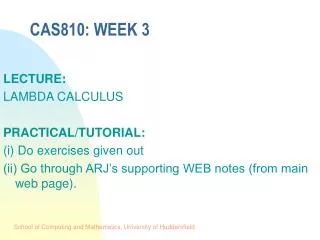
CAS810: WEEK 3 LECTURE: LAMBDA CALCULUS PRACTICAL/TUTORIAL: (i) Do exercises given out (ii) Go through ARJ’s supporting WEB notes (from main web page).
LAMBDA CALCULUS • A Formal System is a formal language together with a well-defined way of “reasoning” with expressions in the language. EG predicate calculus • Lambda Calculus is a formal system designed by Alonzo Church in 1940, developed by Scott and Strachey c.1970.
LAMBDA CALCULUS -- USE • it is a notation for describing the behaviour of functions - it can be used to represent ALL COMPUTABLE FUNCTIONS. • It is used (as other formal systems) to theorise about computation. These theories direct and support work in compiler design, language design, interface design etc .. • LAMBDA CALCULUS expressions are the denotations in our semantic definitions (next week)
LAMBDA CALCULUS -- SYNTAX <lambda-exp> ::= <var> | (<lambda-exp> ) l<var><lambda-exp> | % abstraction <lambda-exp> <lambda-exp> % application NB: • If there are no brackets, expressions are LEFT ASSOCIATIVE - abc = ((a)b)c • We ENRICH syntax with numbers and the function (b->x,y) meaning if b then x else y • Scope rules..
LAMBDA CALCULUS -- WHY? • It has simple, clear structure / syntax providing a simple model of function definition and application • used extensively as a MEANING domain for programming languages • allows us to treat functions as values, and to define functions without giving them a name! EG: lx.x - lambda abstraction - identity function lx.x+1 - lambda abstraction - successor function (lx.x+1)y - application (lx.x+1)(ly.y+1) - application
LAMBDA CALCULUS - substitution The calculus “evaluates” using substitution and use of CONVERSION RULES: • An occurrence of variable x is BOUND in a lambda expression M if lx.N is a sub-expression of M and x occurs within N. Otherwise, the occurrence of x is FREE. • [M/x]N means substitute expression M for all free occurrences of x in N.
LAMBDA CALCULUS - Conversion Rules (i)If y does not occur free in N then lx.N cnva ly[y/x]N (ii) Reduction - (lx.M)N cnvb [N/x]M (iii) Reduction - if x is NOT FREE in M (lx.M)N cnvc M
LAMBDA CALCULUS -- EXAMPLES lx.x - lambda abstraction - identity function lx.x+1 - lambda abstraction - successor function (lx.x+1)y - application (lx.xx)(ly.y) - application recursive functions in enriched syntax.. f = ln.(n=0 -> 1, n*f(n-1))
Introduction to the Semantics of l-calculus Well, you can evaluate them to normal form using the conversion rules… But recursive functions - what do they MEAN?????
Recursive Functions - The Fixed Point Equation E.g. Factorial Function f = ln.(n=0 -> 1, n*f(n-1)) Consider: H = lg.ln.(n=0 -> 1, n*g(n-1)) H f = (lg.ln.(n=0 -> 1, n*g(n-1))) f = ln.(n=0 -> 1, n*f(n-1)) = f by the definition above. Hf = f ... is the fixed point equation
The Fixed Point Equation • Every recursive function f has a corresponding the fixed point equation H f = f where H is constructed as shown in the slide above. So - a non-recursive function which satisfies H f = f can be thought of as the “meaning” f
Problem... But consider f = lx. ly.( x=y -> y+1, f x (f (x-1) (y-1)) ) In this case H has many fixed points !! E.g. lu. lv. u+1 is a fixed point of H. There are many others.
Solving the Fixed Point Equation - “Graphs” of Functions • The Graph of a function f is a list of pairs (n, f n) where n is an input value to f. E.G. Part of the graph for factorial is g = {(0,1), (1,1), (2,2), (3,6), (4,24), (5,120), (6,720) } We can also DEFINE functions using graphs, and approximate recursive functions with them. NB g is an FINITE APPROXIMATION of factorial.
A static solution to the FPE The static solution of the FP equation turns out to be (lots of maths later…): f = Hn(^) as n tends to infinity. eg For the factorial: H = lg.ln.(n=0 -> 1, n*g(n-1)) H ^ = ln.(n=0 -> 1, ^) Graph(H ^) = (0,1), (1, ^), (2, ^), (3, ^), (4, ^)… H H ^ = lg.ln.(n=0 -> 1, n*g(n-1)) (ln.(n=0 -> 1, ^)) Graph(H H ^) = (0,1), (1, 1), (2, ^), (3, ^), (4, ^)…
Example - Conclusion H ^, H H ^, HH H ^, are improving approximations of any recursive function f, where H appears in f’s fixed point equation. SO, the meaning of recursive functions can be given via a “fixed point semantics”. The MYSTERY of recursive functions having infinite fixed points is cleared up - Hn(^) = the least defined fixed point.
Exercises (1) Consider the following Lambda applications: 1.1 (lx.xx)(ly.y) 1.2 (ly.lz.z -> x,y)(lx.ly.xy) 1.3 (lg.ln.(n=0 -> 1, n*g(n-1)) (ly.y+1)) 3 - For each instance of each variable in 1.1-1.3, say whether the instance of the variable occurs free or bound. - Use the conversion rules to find the normal forms for 1.1-1.3. (2) If f is the factorial function, and H f = f, derive H3(^) and H4(^). Hence derive graph(H3(^) ),graph(H4(^) ) and verify that they are improving approximations to f. (3) If H is the general function in the Cmeans of the while loop, derive H1(^) and H2(^) and their graphs. Are they approximations of the while-loop?