Download
1 / 29
330 likes | 544 Views
Introduction to the Ionosphere. Alan Aylward Atmospheric Physics Laboratory,UCL. The F2-Region. 1) Introduction: Structure and Formation of the F-region. Structure. NmF2.

E N D
Introduction to the Ionosphere Alan Aylward Atmospheric Physics Laboratory,UCL
The F2-Region 1) Introduction: Structure and Formation of the F-region Structure NmF2 The F2 layer peak (hmF2) occurs between 250 and 400 km altitude, is higher at night than day and higher at solar maximum conditions. In contrast to the F1 region, the F2 layer is maintained at night. hmF2
Ionosphere composition Major F-region ions is O+, followed by H+ at the top and NO+ and O2+ at the bottom. Note that neutral gas concentration at 300 km is around 108 cm-3, so ion concentrations are 2 orders of magnitude smaller. Negative ions are found only in the lower ionosphere (D region). The net charge of the ionosphere is zero. Dayside ionosphere composition at solar minimum.
Above around 1400 km (day) and 700 km (night), H+ becomes the dominant ion, forming a layer commonly referred to as the Protonosphere. At low latitudes, closed magnetic field lines reach out to several Earth radii, forming flux tubes. This region is referred to as the Plasmasphere.
Ionosphere temperatures In the ionosphere, we distinguish between ion temperatures, Ti, and electron temperatures, Te. Ions and electrons receive thermal energy during the photoionization and lose thermal energy through collisions. Since recombination lifetimes are smaller than the timescale for losing the excess thermal energy, the ion and electron temperatures above 300 km are both larger than the neutral temperatures, Tn :
External coupling of the ionosphere * * * *mainly at high latitudes
Ion/Electron Continuity Equation Loss Production Transport D, E, F1 region:q ~ l(N), Transport mostly unimportant photochemical regime, described by Chapman layers F2 region: Transport matters, q and l(N) no longer dominant optically thin, not Chapman layer
b) Formation of the F2 region *key reactions Photoionization: (λ<911Å) (1) * (λ< 796Å) (2a) (2b) (3) (λ< 1026Å) Dissociative recombination (rapid) : (λ= 6300Å) “Airglow” (4) * (5) * (6) (7)
Radiative recombination (slow) : (8) (7774 Å) Charge transfer: * (9) (10) (11) Ion-atom interchange: (12) * (13) (14)
Electron production profiles Curves are: X(E)…. XEUV (8-140 Å) UV(E).. UV (796-1027 Å) F…….. UV (140-796 Å) E…….. UV(E)+X(E) E+F…. Total (8-1027 Å) Note that peak production occurs near 120 km, whereas the F2 peak is located near 300 km! Loss rate (~[N2]) decreases faster with height than production rate (~[O]) since (O/ N2) increases with height. Ionization peaks occur at optical depth = 1
One can see that the production of ionization depends largely on the [O] density, while photochemical loss is determined by the abundance of N2 and, to lesser degree, O2 (reactions 2a, 2b, 5, 10). This figure shows calculated electron density profiles (Ne) at selected times after photoionization is set to zero. It illustrates the role of photoionization in maintaining the ionosphere.
2) Ion and Electron Dynamics Pressure gradient Lorentz force Gravity Electric field Ions Ion-neutral collisions Ion-electron collisions Electrons
For : Define: Gyrofrequency: Since : In the presence of an E field, particles are partly accelerated and decelerated while gyrating. This causes net drift in the EB direction. Positive and negative charges gyrate in opposite directions around the magnetic field lines.
The motion of charged particles is determined primarily by: • Collisions with the neutral gas particles (at collision frequency v) • External electric field, E • Orientation and strength of magnetic field, B Consider: Frequent particle collisions, B field plays no role, charged particles follow neutral wind. Applies below around 80 km. Case 1: Charged particles affected by E, B and neutral gas motion, leading to interesting behaviour. Applies in E region. Case 2: Charged particles gyrate around B field lines. E field causes EB drift (same direction for ions and electrons). Neutral wind causes UB drift, opposite for ions and electrons, resulting in an electric current. Applies above around 200 km. Case 3:
Idealized electron and ion trajectories resulting from a magnetic field and perpendicular electric field. Charged particles collide with neutrals at regular intervals of 1/v. Numbers in brackets are approximate heights (km) where the situation applies. Note that neutral winds, U, are assumed zero here. Below 180 km ions and electrons drift into different directions. Above 180 km ions and electrons drift in the same direction (EB). Note that the presence of neutral winds however produces a current.
Plasma Diffusion Simplifying the momentum equationand assuming vertical components only, as well as a vertical B field, give: where W are vertical drift velocities. When further assuming mi >> me, Ni = Ne = N, Wi = We = WD (plasma drift velocity) and Wn = 0 (neutral air at rest) and mivin >> meven (electron-neutral collisions less important than ion-neutral collisions) we obtain for the drift velocity:
This expression can be rewritten as: with the following definitions: Plasma temperature Plasma scale height (plasma has average particle mass 0.5*mi, since electron mass is negligible) Plasma diffusion coefficient Assuming Ti = Te = T gives: Ambipolar diffusion coefficient
(D profile) - is complex • extremely energetic particles, • Water cluster ions • Complex chemistry
3) F2 Region Morphology a) Diurnal behaviour • Key features: • Daytime Ne ~ O/N2 • Longevity due to slow recombination (9, 12) • Daytime hmF2 < nighttime hmF2
Neutral wind influence on plasma distribution Nighttime scenario: Neutral winds blow plasma up the magnetic field lines, into regions of lower recombination (hence slow deterioration of F2 layer at night and larger hmF2). Daytime scenario: Neutral winds blow plasma down the magnetic field lines, into regions of stronger recombination. Therefore, hmF2 is lower at day than night. VB Zlargest for dip angleI = 45°
The Earth’s geomagnetic field The Earth’s magnetic field is a tilted, offset dipole field, giving rise to longitude-dependence of the coupling between plasma and neutral winds. Approximate location of geomagnetic poles: 80ºN / 69ºW 79 ºS / 111ºE
The coupling between plasma and neutral winds depends on: • Latitude due to the change of dip angle, being largest at the magnetic pole and smallest over the magnetic equator • Longitude due to the geographic and geomagnetic pole offsets • Local time due to the change of neutral wind direction and electron density (Ne): at night, Ne is lowest, so the slow-down of neutral winds by ions is least effective, giving larger neutral winds at night and stronger vertical plasma drifts. noon midnight noon Therefore, neutral-ion coupling in the F2 region is very complex.
What about the equatorial ionosphere? • Differences are: • B field horizontal • No vertical diffusion, only horizontal • No vertical transport due to meridional winds • What are the consequences of this? Note: hmF2 larger at day than night (other than at mid-latitudes!) Output from International Reference Ionosphere (IRI) model.
Latitudinal structure of Ne at low latitudes • Calculated Ne (in Log10) for December, 20:00 LT. • Note: • hmF2 larger over magn. Equator • build-up of ionization at low latitudes This effect is called the Appleton Anomaly or Fountain Effect. The key to understanding its cause are the zonal neutral winds
Thermospheric winds in the equatorial E region drag ions across the magnetic field lines B, creating during the daytime an eastward dynamo electric field, which is mapped along the magnetic field lines into the F region. This, combined with a northward B field creates an upward EB plasma drift. At dusk, the eastward winds are strongest, producing a particularly strong vertical drift (“pre-reversal enhancement”). The pre-reversal enhance-ment causes Rayleigh-Taylor Instabilities, which may generate small scale structure such as “Equatorial Spread-F”. Note the differences in neutral wind-plasma coupling at low and mid latitudes (shown earlier)!
The equatorial vertical plasma drifts are strongly dependent on neutral winds in the E region. The shown lines are simulations for different tidal diurnal and semidiurnal modes…. …. with considerable impact on the shape and magnitude of the Appleton anomaly. This effect is an example for effective coupling between the thermosphere and ionosphere at different altitudes as well as latitudes!
The impact of vertical drifts on the vertical electron density (Ne) profile at Jicamarca, Peru (xxN/xxW). These simulations show that vertical plasma drifts move the Ne profile up during day and down during night, with respect to the solution without plasma drifts (blue). Including realistic plasma drifts considerably improves the agreement between modeled (red) and observed (black) Ne.