Download
1 / 53
530 likes | 642 Views
Explore numerical schemes for accurate long-term simulation of contaminant migration, including ParSSim and various transport methods - CMM, Godunov, DG. Analyze scaling, dispersion, and computational efficiency.

E N D
Comparison of Numerical Schemes for Accurate Long-term Simulation of Contaminant Migration Krzysztof Banaś1,2, Steve Bryant2 1ICM, Cracow University of Technology 2TICAM, The University of Texas at Austin
Mary F. Wheeler (DIRECTOR) Todd Arbogast Steven Bryant Clint Dawson Rick Dean Eleanor Jenkins Phu Luong Victor Parr Malgorzata Peszynska Béatrice Rivière John Wheeler CSM Researchers + several visitors + 10 graduate students 1999-2000: 5 PhD, 1 MS completed
Overview • Experience with ParSSim • First order Godunov • Higher order Godunov • Characteristics-mixed method • Experience with DG research codes
ParSSimParallel Subsurface Simulator • Multicomponent • logically rectangular 3D • operator splitting • General biogeochemistry • interior point minimization of free energy • explicit integration of kinetics ODEs • Scalable Parallel • domain decomposition (MPI) • SP2, cluster of PCs, T3E, Workstations • dynamic load balancing 1 flowing phase, N stationary phases
ParSSim solution scheme: operator splitting • Solve flow equation • Solve transport equations • Advect • React • rate-limited reactions, mass transfer • thermodynamic equilibrium • Diffuse • Update composition-dependent viscosity, permeability
ParSSim Flow Calculation • Single phase Darcy flow • Logically rectangular, cell-centered finite difference, implicit • Glowinski-Wheeler domain decomposition
ParSSim Transport Biogeo-chemistry Radionuclide decay Injection/extraction wells Linear sorption • Advection step: solve
ParSSim Transport: advection step (1) • Explicit characteristics-mixed method* • Introduce total concentration Ti : • Resulting PDE: • Solve by characteristic tracking: • Extract advected concentrations: • *Arbogast and Wheeler, SIAM J. Numer. Anal. 32 (1995) 404-424
ParSSim Transport: advection step (2) • Higher order Godunov* • Solve directly for advected concentrations • Formally 2nd order, improved by postprocessing step • First order Godunov ( nopostprocessing) • *Dawson, SIAM J. Numer. Anal. 30 (1993) 1315-1332
ParSSim Transport: reaction step • React the advected concentrations • Radionuclide decay • Solve the PDE… • By explicit integration • Biogeochemistry • Solve the PDE… • By explicit integration Equilibrium reactions handled by free energy minimization
ParSSim Transport: diffusion step • Diffuse/disperse the reacted concentrations • Solve the PDE… • Implicitly by
Transport scheme comparisons • Couplex1 • Transport scheme benchmarks* • Moving hill • Curvilinear flow • Mixed waste *http://terrassa.pnl.gov:2080/~kash/workshop/bmark.htm
Couplex1 Simulation 129I plume, Higher Order Godunov solution
Couplex1 Simulation 129I plume, Higher Order Godunov solution
Couplex1 Variant Decrease clay layer diffusion coefficient 1000 times 129I plume, Higher Order Godunov solution
Couplex1 Simulation 129I plume, character-istics-mixed method solution
Couplex1 Simulation 129I plume, Characteristics Mixed Method solution
Couplex1 Variant Decrease clay layer diffusion coefficient 1000 times 129I plume, Characteristics Mixed Method solution Note “hot spot” at clay-limestone boundary
Moving Hill (Benchmark 6) Conservative tracer 5050 grid vx = vy NPe(grid)= 102 NCr = 0.1 y x
http://terrassa.pnl.gov:2080/~kash/workshop/problems/pcl/prob1/ashok1.htmhttp://terrassa.pnl.gov:2080/~kash/workshop/problems/pcl/prob1/ashok1.htm
http://terrassa.pnl.gov:2080/~kash/workshop/problems/pcl/prob1/ashok1.htmhttp://terrassa.pnl.gov:2080/~kash/workshop/problems/pcl/prob1/ashok1.htm
Benchmark 6: Results First order Godunov Higher order Godunov Characteristics-mixed method Discontinuous Galerkin
Benchmark 5 Description 150 x 150 grid zero diffusion solute inlet effluent collection window
Benchmark 5: Tracer Effluent Analytical HOG CMM
Benchmark 5: DG results Results from current research code, courtesy K. Banas
Benchmark 5: Reactive Solute Effluent Analytical, half order HOG
Transport scheme comments • Characteristics-mixed method (CMM) • Minimal numerical dispersion • No CFL constraint (except that arising from domain decomposition) • Good scaling in parallel • Computationally expensive • Higher order Godunov • Locally mass conservative • CFL constraint • More numerical dispersion than CMM • Computationally inexpensive • Discontinuous Galerkin • Even less numerical dispersion than CMM • Subject of current research
DG Methods • Unstructured, non-matchinggrids • Element refinements/de-refinements • Local high order of approximations • Arbitrary tensor coefficients and BC • Locally conservative • Error estimators (for hp adaptivity) • Positive definiteness
3D elements of “arbitrary” shape • Tetrahedral • Prismatic • Hexahedral
hp-adaptivity • Order of approximation specified element-wise • Isotropic element divisions • Anisotropic element divisions
Iterative linear equations solver • Large, sparse, non-symmetric, positive definite systems of linear equations • Single level GMRES as default solver • Multi-level GMRES for elliptic problems • Preconditioning by ILU, domain decomposition • Implementation based on block Gauss-Seidel iterations • Easy parallelization
Application to subsurface flows • Single phase flow • Miscible displacement • Two-phase flow • Interfaces with IPARS framework
Miscible Displacement Concentration Front