Download
1 / 40
400 likes | 487 Views
Explore the predictive power of the Vegas line and factors influencing college football wins. Authors delve into models, data sources, and implications for coaching and recruiting.

E N D
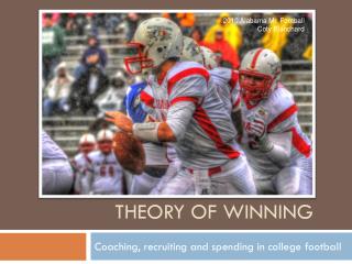
2010 Alabama Mr. Football Coty Blanchard Theory of winning Coaching, recruiting and spending in college football
Table of Contents • Introduction • How to predict a win • Data sources • Initial Model • Out of sample prediction • Practical applications • Next steps Jason Campbell, Auburn University
Authors Introduction • McDonald “Mac” Mirabile • Manager of Strategic & Financial Analysis at WWF • Undergraduate and graduate thesis on the predictors of a successful transition from college to NFL • Prior academic publications on topics such as biases in college football polls, the NFL Rookie Cap, the Wonderlic Test, and the Peer Effect in the NFL draft • Mark Witte • Assistant Professor at College of Charleston • Generally awesome guy
Topic Introduction • The importance of winning in college • Shapes alumni support, attendance • Influences quality of recruiting • Self-enforcing cycle
How to predict a win • Vegas point spread, totals, and money line theoretically capture all available information under the efficient market hypothesis (EMH) • Existing literature consistently enforces EMH, though there are some published examples of deviations and profitable strategies within wagering markets • Within the framework of this paper, we will assume EMH holds within college football wagering markets and will measure the success of our developed models relative to the baseline Vegas model
Predicting Wins with the Vegas Line • Bubble chart illustrates the home team’s winning percent by the Vegas Line, with the size of the bubble based on the number of observations
Predicting Wins with the Vegas Line • Bar chart of home team’s winning percentage by the Vegas line
The Vegas Line model • Home Win (0,1) = b1*Line + error • This model within our data explains 29% of the variation in wins (Pseudo R2). • The line coefficient is 0.1091, with a standard error of 0.00437, and an Odds Ratio of 1.115 • Interpretation: for each additional point a team is favored, their odds of winning increase by 11.5% • Non-linear model shows similar results
Improving the Vegas Line model • Can it be done, or does the Vegas line incorporate all publically available information? • To test this, we added several variables: • Home, Away win and losing streaks • Home, Away AP Rankings, Top 25 matchups • Dummy variables for conference games, neutral field matchups, and night games • Distance between schools, stadium size, rivalry information • Conference dummy variables
Improving the Vegas Line model Effect DF Wald Pr > ChiSq Line 1 285.4691 <.0001 ETP 1 1.1213 0.2896 HWS 1 0.522 0.47 HLS 1 0.8024 0.3704 AWS 1 1.8483 0.174 ALS 1 0.1004 0.7513 Hrank 1 0.7195 0.3963 Arank 1 0.1588 0.6903 HNR 1 1.591 0.2072 ANR 1 1.5452 0.2138 TrueT25 1 0.2535 0.6146 ConfGame 1 0.003 0.9566 Neutral 1 0.001 0.9743 Nightgame 1 0.3414 0.559 Stadium 1 1.078 0.2992 Distance 1 0.0145 0.9042 Rivalry 2 2.0766 0.3541 Conf 12 11.5154 0.4853 • Table on left shows these additional variables and a their corresponding Wald Chi2 statistics • The Vegas line successfully incorporates all available information. • Adding more explanatory variables does not improve the model’s fit. • None of the added variables are statistically significant as their importance is already captured in the Line variable.
Data Sources • To develop a model of winning without utilizing the Vegas line, the authors gathered data on the following topics: • Game-specific factors • Institutional factors/history • Team player composition/recruiting • Team coach factors/history • We will discuss the collection and organization of this data next
Game-specific Factors • Matchup data comes from Covers.com • Data includes game location, time, day, conference information • Each matchup (home vs away) is one observation in the dataset • There are about 500 games per season
Institutional Factors & History • Historical team performance comes from CFBDatawarehouse.com • University football team expenditure and student body size data come from the Equity in Athletics website • Each of these variables is reported for a particular year (e.g., Michigan’s historical team performance through 2007 and their team expenditure data for the 2008 season would all be used as predictors for the 2008 season matchups)
Team player composition and recruiting • Class recruiting data comes from Rivals.com, Scouts.com, and Prepstar.com • Recruiting classes in 2005 (RS-Senior), 2006 (Senior / RS-Junior), 2007 (Junior, RS-Sophomore), 2008 (Sophomore, RS-Freshman), an 2009 (Freshman) are used as predictors for the 2009 season matchups. • Due to the NFL draft, transfers, and general attrition, these variables are imperfect measures of the talent comprising a team in a particular season
Team coach factors and history • Historical coach performance comes from CFBDatawarehouse.com • Coach biographical information comes from various university athletics department websites • Each of these variables is reported for a particular year (e.g., Michigan’s coach’s historical performance through 2007 would be used as a predictor for the 2008 season matchups)
Initial Model • Matchup-specific variables: • Stadium Size • Home team student size • School-specific variables: • Cumulative Team Win Pct Diff • Log Diff of Total Team expenditures • Team-specific variables (Difference home – away): • Scouts.com weighted average class ranking • Coach-specific variables (Difference home – away) : • First year head coach Home team dummy • First year head coach Away team dummy • Coach age • Coach experience (assistant + HC) • Head coach seasons • Lifetime Coach Win Pct Diff • Years as NFL player • Home team’s head coach minority dummy • Away team’s head coach minority dummy N: 2,948R-Square: .215
Initial Model - Interpretations • Matchup-specific variables: • Stadium Size – for every additional 10,000 seats, the home team is 4% more likely to win • (also considered game time, location, rivalry variables) • School-specific variables: • Log Diff of Total Team expenditures – the odds ratio of the % difference (home/away) in team spending of 2.5 suggests that a team spending 100% more (twice as much) is 150% more likely to win, (Alternative, equivalent interpretation: odds of winning increase 15% for each 10% increase in excess of your opponent’s expenditures) • Team-specific variables (all Difference home – away) : • Scouts.com average class ranking – for each unit increase in average class ranking between the home and away, the home team is 1% more likely to win • Coach-specific variables (all Difference home – away) : • First year head coach dummy variables – marginally significant and coefficients in the direction one would expect • Diff in HC’s ages – for each additional year in age difference b/w the Home and Away team’s coach, the home team is 1% less likely to win • Diff in HC’s cumulative Win % – for each 1% difference in lifetime win percentage between the home team’s HC and the away team’s HC, the home team is about 6% more likely to win • Years as NFL player – for each additional year of NFL playing experience between the home team’s HC and the away team’s HC, the home team is about 4% less likely to win • Home team Head Coach Minority – minority coaches are 42% less likely to win than non-minority coaches at home • Away team Head Coach Minority – home teams are 87% more likely to win when playing against a minority coach
Out of Sample prediction Both models have comparable in and out of sample performance
Out of Sample by Line • Vegas line does a better job predicting everything except games where the line is between -2 and +2
2009 Season (SEC results) • Data from 2004-2008 used to develop the model • Data from 2009 used in an out-of-sample validation Note: Non Div1A opponents not scored/modeled
Practical Applications • Predict 2010 season results – conference standings, national champion, before a single game has been played
Next steps • What can be added to the model? • New sources of data (attendance, compensation/bonus – impute missing values based on relative rank of team within conference?) • Additional data cleanup (game time, more years 2001-2003) • Different estimation methodologies
Who is hiring minority coaches? • The coach is more likely to be young (see coach_age), belong to a historically crappy program (Cum_WinPCT_School_H) as well as belong to a recently crappy program (MA5_Win_PCT_School_H) of relatively newer schools (School_Seasons_H) and larger schools (Stadium).
Predicting recruiting classes • GLM estimation of dependent variable: Scouts class ranking • Previous year and 5-year MA Win % impact recruiting • Previous classes are also good predictors of current year’s class ranking • Conference impacts recruiting Alabama (2010) = 43.4 – (9.7*1) – (15.5*.77) + (.27*2) + (.18*1) + (.1*22) + (.13*18) – 21.8 = 3 (Actual rank 4) Auburn (2010) = 43.4 – (9.7*.615) – (15.5*.66) + (.27*16) + (.18*18) + (.1*6) + (.13*9) – 21.8 = 15 (Actual rank 5) Vanderbilt (2010) = 43.4 – (9.7*.167) – (15.5*.38) + (.27*72) + (.18*74) + (.1*87) + (.13*61) – 21.8 = 63 (Actual rank 61)
Other considerations (backup slide) • Off the field model .18 • On the field model .26 • Are the coefficients robust? • Future problems: things that recruits like – new stadiums, new weight rooms, facilities • Could we do a recruiting paper modeled on NCAA football recruiting info – coach history, academic prestige, location, tv time, etc
Out of Sample prediction (intercept) Both models have comparable in and out of sample performance
Friday • Meet with profs about research • Present to a class • Lunch • Seminar presentation • Dinner
Models • To begin, we will look at each of these data sources and its relationship to our outcome variable individually. • Because each of these data sources is described with dozens of potential variables, this initial modeling will inform our final set of models where data from all possible sources are considered in development. • All models are developed using a Logit function as our outcome variable, Home Win, is binary. We will discuss the resulting coefficients as Odds Ratios to aid interpretation.
Model 1: Game specific factors • Other considered variables • Distance b/w schools • Rivalry game (major/minor/none) • Other variables to consider in the future: • Game-time (need to clean some data)
Model 2: Institutional factors & history • Other considered variables • Other variables to consider in the future: