Seismic attribute-assisted interpretation of incised valley fill episodes: A case study

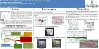
1. Seismic attribute-assisted interpretation of incised valley fill episodes: A case study of Anadarko Basin Red Fork interval. Yoscel Suarez*, Chesapeake Energy and The University of Oklahoma, USA Kurt J. Marfurt, The University of Oklahoma, USA Mark Falk, Chesapeake Energy, USA Al Warner , Chesapeake Energy, USA III II V Abstract Previous Work Methodology Pink Lime II Middle Red Fork V II III Lower Red Fork Using Peyton et al’s (1998) work as a starting point we generated similar displays of conventional seismic profiles and well x-sections that will become the bases of our research efforts. Figure 8 shows the geometry and extents of the different episodes of the Red Fork incised valley system based on well data interpretation and conventional seismic displays. This map will be compared to the different seismic attributes to calibrate their response. Figure 9 (a,b) show couple of well x-sections and their corresponding seismic profiles that supported the valley-fill stages map in Figure 8. Seismic attributes have undergone rapid development since the mid 1990s. In lieu of the horizon-based spectral decomposition based on the discrete Fourier transform, we use volumetric-based spectral decomposition based on matched pursuit and wavelet transforms (e.g. Liu and Marfurt,2007) . Other edge-sensitive attributes include more modern implementations of coherence, long-wavelength Sobel filters, and amplitude gradients. Figure 10 shows a horizon slice at the Red Fork level. Note that on conventional data the channel complex is identifiable. However, the use of seismic attributes may help delineate in more detail the different episodes within the same fluvial system and better define channel geomorphology. We will compare different edge detection algorithms and the advantages and disadvantages that each of them provides to the interpreter. Also, matching pursuit spectral decomposition results will be presented as well as combinations of Relative Acoustic Impedance and semblance that provide helpful information in the interpretation of this dataset. In 1998 Lynn Peyton, Rich Bottjer and Greg Partyka published a paper in the Leading Edge describing their use of coherency and spectral decomposition to identify valley fill in the Red Fork interval in the Anadarko Basin. Their work help them identify five valley-fill sequences in order to find optimum reservoir intervals and to reduce exploration risk . Due to the discontinuity of the valley-fill episodes the mapping of such events by using conventional seismic displays is extremely challenging. Figure 3 shows one of the stratigraphic well cross-section presented by Peyton et al where the discontinuities of this complex are evident. Figure 4 shows a seismic profile that parallels the wells cross-section highlighting the same stages. The seismic section is flattened in the Novi. By generating horizon slices in the coherency volume they were able to identify and delineate the main geometries of the incised valley (Figure 5). The event used to generated the horizon slice is the Skinner Lime above the Red Fork interval. In their workflow they also estimated the spectral decomposition. They found that the 36 Hz component best represented the different valley-fill stages (Figure 6). By combining the well-data with the information from the seismic attributes they were able to delineate the extents of the different valley –fill episodes (Figure 7) and generate and integrated interpretation of the system. Discrimination of valley-fill episodes and their lithology has always posed a challenge for exploration geologists and geophysicists, and the Red Fork sands in the Anadarko Basin do not fall outside of this challenge. The goal of this study is to take a new look at seismic attributes given the considerable well control that has been acquired during the past decade. By using this well understood reservoir as a natural laboratory, we calibrate the response of various attributes to a well-understood incised valley system. The extensive drilling program shows that seismic data has difficulty in distinguishing shale episodes vs. sand episodes, where the ultimate exploration goal is to find productive valley fill sands. Since original work done in 1998 both seismic attributes and seismic geomorphology have undergone rapid advancement. The findings of this work will be applicable to nearby active areas as well as other intervals in the area that exhibit the same challenges. The surveys are located in west central Oklahoma. They were shot by Amoco from 1993- 1996 and later merged into a 136 sq.mi. survey. In 1998, Chesapeake acquired many of Amoco’s Mid-continent properties including those discussed by Peyton et al. (1998). In this study we present alternative seismic attribute-assisted interpretation workflows that show the potential information that each of the geometric and amplitude-based attributes offer to the interpreter when dealing with Red Fork valley-fill episodes in the Anadarko Basin. It is important to mention that one of the biggest challenges of this dataset is the acquisition footprint, which contaminates the data and limits the resolution of some of the seismic attributes. A Figure 4. Seismic profile associated to the prior cross-section. Flattened in the Novi interval Figure 3. Stratigraphic cross-section Red Fork valley –fill complex Geological Framework Phase II Phase III Phase V A’ The Pennsylvanian incised valley sequence associated with the Red Fork interval has, throughout most of its extent, three major events or facies (Phase I, II, and III) which can be differentiated by log signatures, production characteristics, and gross geometry. Two additional events (Phase IV and V) are present in the eastern and northeastern headward portion of the valley, also recognizable by log signature and gross geometry. The multi phase events of the Upper Red Fork Valley system were most likely caused by repeated sea level changes resulting from Pennsylvania glacial events that were probably related to the Milankovitch astronomical cycles including the changing tilt of the earth’s axis and eccentricity of the earth’s elliptical orbit. Figure 8. Red Fork incised valley geometries and valley-fill episodes Figure 10. Conventional seismic horizon slice at the Red Fork level. The channel discernible although signal/noise ratio is affected by acquisition footprint Phase I is the earliest valley event and represents the narrow, initial downcutting of the valley sequence. Where present (a considerable portion of Phase I has been eroded by later events), the rocks are generally poorly correlative shales, silts, and tight sandstones overlying a basal “lag” deposit. Phase II generally has a much wider areal distribution (up to four miles) with a variety of valley fill facies deposited which record a period of valley widening and maturation. Logs over Phase II rocks illustrate a classic fining upward pattern and shale resistivities of 10 or more ohms. Figure 5. Coherency horizon slice at the Red Fork level Phase III rocks record the last major incisement within the valley and occur within a narrow (0.25-.05 mile wide) steep walled system that is correlative for 70 miles. This rejuvenated channel actually represents the final position of the Phase II river before base level was lowered and renewed downcutting began. Phase III reservoirs are primarily thick, blocky, porous sands at the base of the sequence that have been backfilled, reworked, and overlain by low resistivity marine shales deposited by a major transgression which drowned the valley sequence. a) Figure 9. a) Red Fork stratigraphic cross-section. b) Seismic profile showing the stratigraphic interpretation derived from the well data Phase IV records a modest regression at the end of Phase III marine shale deposition. Phase IV rocks are characterized by thin, tight, interbedded sands and shales with a coal or coaly shale near the base. This facies is interpreted as an elongated lagoon/ coal swamp or possibly bay head delta as it often extends beyond the confines of the deeper valley. The Induction log signature is a very distinct “serrated” pattern with a “hot” gamma ray near the base identifying the coal or coaly shale. Phase V the last event before the transgression that deposited the Pink. It’s primary significance is that it either partially or completely eroded much of the Phase III Valley event. Phase V rocks are poorly developed, non productive sand and shales which also have a characteristic log signature. The geological framework summary is courtesy of Al Warner. Senior Geologist at Chesapeake Energy b) Figure 7. Spectral decomposition (36 Hz) horizon slice at the Red Fork level with interpretation. Figure 6. Spectral decomposition (36 Hz) horizon slice at the Red Fork level

2. Seismic attribute-assisted interpretation of incised valley fill geometries: A case study of Anadarko Basin Red Fork interval. Yoscel Suarez*, Chesapeake Energy and The University of Oklahoma, USA Kurt J. Marfurt, The University of Oklahoma, USA Mark Falk, Chesapeake Energy, USA Al Warner , Chesapeake Energy, USA Seismic Attribute Generation Edge Detection Relative Acoustic Impedance The Relative Acoustic Impedance (RAI) is a simplified inversion. This attribute is widely used for lithology discrimination and as a thickness variation indicator. Since the RAI enhances impedance contrast boundaries, it may help delimit different facies within an incised valley-fill complex. Figure 15 shows the better delineation of the different valley-fill episodes. The impedance amplitude variations within the system may be correlated to sand/shale ratios. Higher values of RAI seem to be related to sandier intervals (black arrow). Coherence According to Chopra and Marfurt (2007) coherence is a measure of similarity between waveforms or traces. Peyton et al. (1998) showed the value of this edge detection attribute to identify channel boundaries in the Red Fork level. Figure 11 shows the results of the modern coherence algorithm and the interpretation. The modern coherence algorithm is slightly superior. It shows additional features (blue arrows), and enhances the edge of Phase II (pink arrow). It also shows that the current outlines of Phase II could be modified in the encircled areas. Conclusions Figure 15. Relative Acoustic Impedance (RAI) at the Red Fork level. This study has identified correlations between attribute expressions of Red Fork channels that can be applied to underexploited exploration areas in the Mid-continent, and to fluvial deltaic channels in Paleozoic rocks in general. When it comes to answer the key questions discussed at the beginning of this paper, we learned that the coherence and energy weighted attributes help improve the resolution of subtle features like small channels and channel levees. They also help differentiate the cutbank from the gradational inner bank. It is also evident from this study that even though there have been some improvements in the coherence routines, the differences between current algorithms with the ones applied by Peyton et al. in 1998 are minimal. Additionally, detailed channel geomorphology and lithology discrimination were possible by introducing the spectral decomposition and relative acoustic impedance attributes in the analysis. On one hand, the use of spectral decomposition helped define different facies within the channel system and increased the resolution of channel boundaries. On the other hand, the variations in the RAI values were found to be correlative to lithology infill, for instance higher values of RAI show direct relationship to shalier intervals within the channel complex. One of the key findings of this study is the great value that blended images of attributes bring to the interpreter. Such technology was not available ten years ago. But today, by combining multiple attributes, fluvial facies delineation is possible when co-rendering edge detection attributes with lithology indicators. It is important to mention that the signal/noise ratio of the data is a key factor that will determine the resolution and quality of the seismic attribute response. In this study, curvature did not provide images of additional interpretational value. These unsatisfactory results may be related to acquisition footprint contamination. Therefore, footprint removal methods will be performed in an attempt to enhance signal-to-noise ratio. Figure 11. Modern coherency horizon slice at the Red Fork level Energy Weighted Coherent Amplitude Gradients Chopra and Marfurt (2007), by using a wedge model, demonstrate that waveform difference detection algorithms are insensitive to waveform changes below tuning frequencies. In this study the energy ratio coherence, defined by the coherent energy normalized by the total energy of the traces within the calculation window, and the Sobel coherence, which is a measure of relative changes in amplitude were used. Figure 12 shows a horizon slice of the energy ratio coherence and the Sobel coherence at the Red Fork level. The results from these two energy weighted routines are very similar to the coherence attribute, however the level of detail of the coherency algorithm is greater in the encircled areas. Even though both algorithms show similar features, the Sobel coherence seems to be more affected by the acquisition footprint than does the energy ratio coherence. Seismic Attribute Blending Peak Frequency and Peak Amplitude Displays Liu and Marfurt (2007) show that by combining the peak frequency and peak amplitude volumes extracted from the spectral decomposition analysis, the interpreter can identify highly tuned intervals. Low peak frequency values correlate with thicker intervals and high peak frequencies with thinner features. Figures 16 (a,b) show the peak frequency and peak amplitude volumes respectively. Figure 16(c) shows the combination of both displays, which simplifies the interpretation of multiple volumes of data. Figure 16(d) shows the blended image with the overlain geological interpretation. This combination iof attributes shows a better definition of the Phases boundaries especially the Phase II in the NW corner of the survey, in between the two valley branches. The changes in facies within the Phase V are evident in the southernmost green arrow. The differentiation between the Phase III and Phase V is sharper (northernmost green arrow). Outside of the incised valley system the lithology relationship with frequency is still unclear. The dashed orange lines show the proposed changes to the Phase II outline. Figure 12. Other modern edge-detector attributes: a) Sobel coherence. b) Energy ratio coherence Curvature Although successful in delineating channels in Mesozoic rocks in Alberta, Canada (Chopra and Marfurt, 2008), for this study, volumetric curvature does not provide images of additional interpretational value. While the Red Fork channel boundaries can be delineated using this attribute (Figure 13), the results shown by the coherence and spectral decomposition are superior. In this situation the acquisition footprint negatively impacts the lateral resolution quality of the attribute. Blue arrows indicate channel edges. Acknowledgments Figure 16. Peak Frequency and Peak Amplitude analysis at the Red Fork level. (a) Peak Frequency volume, red corresponds to higher frequencies. (b) Peak Amplitude volume, white corresponds to higher peak amplitude values. (c) Peak frequency and peak amplitude blended volume. The co-rendered image shows valley-fill boundaries. (d) co-rrendered image with interpretation We thank Chesapeake Energy for their support in this research effort. We give special thanks to Larry Lunardi, Carroll Shearer, Mike Horn, Mike Lovell and Travis Wilson for their valuable contribution and feedback. And to my closest friends Carlos Santacruz and Luisa Aurrecoechea for cheering me up at all times. Figure 13. Other modern edge-detector attributes: a) Sobel coherence. b) Energy ratio coherence Amplitude Variability Semblance of the Relative Acoustic Impedance Chopra and Marfurt (2007) define semblance as “the ratio of the energy of the average trace to the average energy of all the traces along a specified dip.” Since RAI has sharper facies boundaries the semblance computed from RAI should be crisper than semblance computed from the conventional seismic. Figure 17 shows the value of combining these attributes. Outside of the channel complex the lithology relationship with frequency is still unclear(red arrow). The yellow arrow points to a potential fluvial channel outside of the incised valley-system. The dashed orange lines show the proposed changes to the Phase II outline. Spectral Decomposition Matching pursuit spectral decomposition was used to generate individual frequency volumes as well as peak amplitude and peak frequency datasets. Castagna et al. (2003) discuss the value of using matching pursuit spectral decomposition and how we can associate different “tuning frequencies” to different reservoir properties like fluid content, thickness and/or lithology. Figure 14 shows a matching pursuit 36 Hz spectral component at the Red Fork level. The level of detail using matching pursuit spectral decomposition is superior to that provided by the DFT Figure 17 a) the Semblance of the RAI and b) RAI and RAI semblance blended image. The combination of both attributes helps delineate Relative Acoustic Impedance boundaries. Figure 14. 36 Hz matching pursuit spectral decomposition. Note the enhanced level of detail offered by the matching pursuit spectral decomposition. a) without geological interpretation b) with geological interpretation