Download

1 / 15
150 likes | 257 Views
Reduction of Variables in Parameter Inference Günter Zech, Universität Siegen.

E N D
Reduction of Variables in Parameter Inference Günter Zech, Universität Siegen Motivation: Parameter fitting from multidimensional histograms often suffers from statistical difficulties due to low numbers of events per bin. (Relevant if data have to be compared to a Monte Carlo simulation and therefore a simple likelihood fit is not possible.) Goal:Reduce the dimensionality without loss of information Phystat2005, Oxford G. Zech, Universitaet Siegen
Historical example Determination of V/A coupling in t-decay at PETRA reaction: distribution: 1 parameter, 6 variables, about 30 events with 3 bins per variable we get about 2 events / bin (A simple likelihood fit was not applicable due to acceptance corrections by Monte Carlo simulation.) Some groups fitted the distribution. Phystat2005, Oxford G. Zech, Universitaet Siegen
Simple case: 2 random variables, 1 linear parameter Define new variables: We get The only relevant variable isu (The analytic expression of g(u,v|q) is not required!) The generalization to more than 2 variables is trivial Phystat2005, Oxford G. Zech, Universitaet Siegen
Example: Experimental data xi,yi,ziui MC: generate x,y,z u Perform a likelihood fit to a superposition of the two MC distributions of u Phystat2005, Oxford G. Zech, Universitaet Siegen
Nonlinear parameter dependence Linearize, approximate by Taylor expansion at first estimate q0 of q, fit Dq Several parameters We need one variable per parameter (makes only sense if initially the number of variables is larger than the number of parameters) Phystat2005, Oxford G. Zech, Universitaet Siegen
Can we do any better? Approximate a sufficient statistic Example: distorted lifetime distribution (exponential) Mean value of experimental data is still approximatively sufficient. Compute relation between observed and true value by Monte Carlo simulation. [Full detector simulation for t0 t0‘ Reweight MC events t(t‘)] Phystat2005, Oxford G. Zech, Universitaet Siegen
Monte Carlo curve Data tobserved + error estimated t + error Phystat2005, Oxford G. Zech, Universitaet Siegen
Approximatelikelihood estimate • pdf: • (x, q could be multidimensional) • ignore acceptance and resolution effects and determine parameters + errors from a likelihood fit • to the the observed data • generate Monte Carlo events for • loop , re-weight events by • and perform likelihood fit • correct experimental value Phystat2005, Oxford G. Zech, Universitaet Siegen
Remarks: • The fit of the experimental data to the uncorrected pdf provides an approximate estimate for the parameters. • Other sufficient statistics may be used, which do not require a likelihood fit. • In some cases where the resolution is bad the pdf may be undefined for some experimental values of x. Shifting or scaling of data helps. • For more than 2 parameters it is tedious to determine the relation between true and observed parameter values. • In case acceptance and resolution effects are very large, we may have to take them into account. How? Phystat2005, Oxford G. Zech, Universitaet Siegen
Acceptance effects Acceptance effects do not necessarily spoil the method. Example: The mean value of lifetimes remains a sufficient statistic when the exponential is truncated at large times. Phystat2005, Oxford G. Zech, Universitaet Siegen
General case (only losses, no resolution effects): a(x) = acceptance Likelihood: The last term is a constant and can be discarded. The integrated acceptance A(q) has to be estimated by a Monte Carlo simulation. (Table or approximated by an analytic expression) The acceptance estimate may be crude. Approximations reduce the precision but do not bias the result. The simulation q(qobseved) takes care of everything. Phystat2005, Oxford G. Zech, Universitaet Siegen
Resolution effects • Can normally be neglected (remember: approximation do not bias the result) • When non-negligible: • Perform binning-free unfolding (see my SLAC contribution) • Do a likelihood fit with the unfolded data • simulate complete procedure with MC (may require some CPU power.) Phystat2005, Oxford G. Zech, Universitaet Siegen
Approximate estimators for linear and quadratic pdfs • (in case acceptance and resolution effects are small) • p.d.f.: • Asume a=a0+a, b=b0+b, f f0(x)=f(x |a0,b0) • a, b small • Neglect quadratic terms in a, b • (very fast, could be used online) Phystat2005, Oxford G. Zech, Universitaet Siegen
Summary • Method 1: Reduction of variables • The Number of variables can be reduced to the number of parameters. This simplifies a likelihood inference of the parameters if the number of parameters is less than the number of variables. • Goodnes-of-fit can be applied to the new variable(s) (simplifies g.o.f.) • Acceptance and resolution effects can be taken into account in a similar way as in the second method. (has not been demonstrated) Phystat2005, Oxford G. Zech, Universitaet Siegen
Method 2: Use of an approximatly sufficient statistic or likelihood estimate • No large resolution and acceptance effects: • Perform fit with uncorrected data and undistorted likelihood function. • Acceptance losses but small distortions: • Compute global acceptance by MC and include in the likelihood function. • Stong resolution effects: • Perform crude unfolding. • All approximations are corrected by the Monte Carlo simulation. • The loss in precision introduced by the approximations is usually completely negligible. Phystat2005, Oxford G. Zech, Universitaet Siegen