Parallel Sorting
Parallel Sorting. James Demmel www.cs.berkeley.edu/~demmel/cs267_Spr09. Some Sorting algorithms. Choice of algorithm depends on Is the data all in memory, or on disk/tape? Do we compare operands, or just use their values? Sequential or parallel? Shared or distributed memory? SIMD or not?

Parallel Sorting
E N D
Presentation Transcript
Parallel Sorting James Demmel www.cs.berkeley.edu/~demmel/cs267_Spr09 CS267 Lecture 24
Some Sorting algorithms • Choice of algorithm depends on • Is the data all in memory, or on disk/tape? • Do we compare operands, or just use their values? • Sequential or parallel? Shared or distributed memory? SIMD or not? • We will consider all data in memory and parallel: • Bitonic Sort • Naturally parallel, suitable for SIMD architectures • Sample Sort • Good generalization of Quick Sort to parallel case • Radix Sort • Data measured on CM-5 • Written in Split-C (precursor of UPC) • www.cs.berkeley.edu/~culler/papers/sort.ps CS267 Lecture 24
LogP – model to predict, understand performance • Latency in sending a (small) message between modules • overhead felt by the processor on sending or receiving msg • gap between successive sends or receives (1/BW) • Processors P ( processors ) P M P M P M ° ° ° o (overhead) o g (gap) L (latency) Limited Volume Interconnection Network ( L/ g to or from a proc) a b
140.00 Bitonic 1024 120.00 Bitonic 32 100.00 80.00 Column 1024 us/key 60.00 Column 32 40.00 Radix 1024 20.00 Radix 32 0.00 Sample 1024 16384 32768 65536 131072 262144 524288 1048576 Sample 32 N/P Bottom Line on CM-5 using Split-C (Preview) • Good fit between predicted (using LogP model) and measured (10%) • No single algorithm always best • scaling by processor, input size, sensitivity • All are global / local hybrids • the local part is hard to implement and model Algorithm, #Procs CS267 Lecture 24
Bitonic Sort (1/2) • A bitonic sequence is one that is: • Monotonically increasing and then monotonically decreasing • Or can be circularly shifted to satisfy 1 • A half-cleaner takes a bitonic sequence and produces • First half is smaller than smallest element in 2nd • Both halves are bitonic • Apply recursively to each half to complete sorting • Where do we get a bitonic sequence to start with? 0 0 1 1 1 0 0 0 0 0 0 0 1 0 1 1 0 0 0 0 1 0 1 1 0 0 0 0 0 1 1 1 CS267 Lecture 24
Bitonic Sort (2/2) • A bitonic sequence is one that is: • Monotonically increasing and then monotonically decreasing • Or can be circularly shifted to satisfy • Any sequence of length 2 is bitonic • So we can sort it using bitonic sorter on last slide • Sort all length-2 sequences in alternating increasing/decreasing order • Two such length-2 sequences form a length-4 bitonic sequence • Recursively • Sort length-2k sequences in alternating increasing/decreasing order • Two such length-2k sequences form a length-2k+1bitonic sequence (that can be sorted) CS267 Lecture 24
Bitonic Sort for n=16 – all dependencies shown Similar pattern as FFT: similar optimizations possible Block Layout • remaining stages involve • Block-to-cyclic, local merges (i - lg N/P cols) • cyclic-to-block, local merges ( lg N/p cols within stage) lg N/p stages are local sort – Use best local sort
Bitonic Sort: time per key Measured Predicted using LogP Model #Procs 80 80 70 70 512 60 60 256 50 50 128 40 40 us/key us/key 30 30 64 20 20 32 10 10 0 0 16384 32768 65536 16384 32768 65536 131072 262144 524288 131072 262144 524288 1048576 1048576 N/P N/P CS267 Lecture 24
Sample Sort 1. compute P-1 values of keys that would split the input into roughly equal pieces. – take S~64 samples per processor – sort P·S keys (on processor 0) – let keys S, 2·S, . . . (P-1)·S be “Splitters” – broadcast Splitters 2. Distribute keys based on Splitters Splitter(i-1) < keys Splitter(i) all sent to proc i 3. Local sort of keys on each proc [4.] possibly reshift, so each proc has N/p keys If samples represent total population, then Splitters should divide population into P roughly equal pieces CS267 Lecture 24
Sample Sort: Times Measured Predicted # Processors 30 30 25 25 512 20 20 256 128 15 15 us/key us/key 64 10 10 32 5 5 0 0 16384 32768 65536 16384 32768 65536 131072 262144 524288 131072 262144 524288 1048576 1048576 N/P N/P CS267 Lecture 24
30 Split 25 Sort 20 Dist 15 us/key Split-m 10 Sort-m 5 Dist-m 0 16384 32768 65536 131072 262144 524288 1048576 N/P Sample Sort Timing Breakdown Predicted and Measured (-m) times CS267 Lecture 24
Sequential Radix Sort: Counting Sort • Idea: build a histogram of the keys and compute position in answer array for each element A = [3, 5, 4, 1, 3, 4, 1, 4] • Make temp array B, and write values into position B = [1, 1, 3, 3, 4, 4, 4, 5] • Cost = O(#keys + size of histogram) • What if histogram too large (eg all 32-bit ints? All words?) CS267 Lecture 24
Radix Sort: Separate Key Into Parts • Divide keys into parts, e.g., by digits (radix) • Using counting sort on these each radix: • Start with least-significant sort on 3rd character sort on 2nd character sort on 1st character • Cost = O(#keys * #characters) CS267 Lecture 24
Histo-radix sort Per pass: • compute local histogram – r-bit keys, 2r bins 2. compute position of 1st member of each bucket in global array – 2r scans with end-around 3. distribute all the keys Only r = 4, 8,11,16 make sense for sorting 32 bit numbers P n=N/P 2 2r 3 CS267 Lecture 24
Histo-Radix Sort (again) Local Data Local Histograms P • Each Pass • form local histograms • form global histogram • globally distribute data CS267 Lecture 24
Predicted Measured 140 140 120 120 100 100 80 80 us/key us/key 60 60 40 40 20 20 0 0 16384 32768 65536 16384 32768 65536 131072 262144 524288 131072 262144 524288 1048576 1048576 N/P N/P Radix Sort: Times # procs 512 256 128 64 32 CS267 Lecture 24
Radix Sort: Timing Breakdown Predicted and Measured (-m) times CS267 Lecture 24
Local Sort Performance on CM-5 Entropy = -Si pi log2 pi , pi = Probability of key i Ranges from 0 to log2 (#different keys) (11 bit radix sort of 32 bit numbers) 10 9 Entropy in Key Values 8 7 31 6 25.1 µs / Key 16.9 5 10.4 4 6.2 3 <--------- TLB misses ----------> 2 1 0 15 20 0 5 10 Log N/P CS267 Lecture 24
Radix Sort: Timing dependence on Key distribution Entropy = -Si pi log2 pi , pi = Probability of key i Ranges from 0 to log2 (#different keys) Slowdown due to contention in redistribution CS267 Lecture 24
140.00 Bitonic 1024 120.00 Bitonic 32 100.00 80.00 Column 1024 us/key 60.00 Column 32 40.00 Radix 1024 20.00 Radix 32 0.00 Sample 1024 16384 32768 65536 131072 262144 524288 1048576 Sample 32 N/P Bottom Line on CM-5 using Split-C • Good fit between predicted (using LogP model) and measured (10%) • No single algorithm always best • scaling by processor, input size, sensitivity • All are global / local hybrids • the local part is hard to implement and model Algorithm, #Procs CS267 Lecture 24
Sorting Conclusions • Distributed memory model leads to hybrid global / local algorithm • Use best local algorithm combined with global part • LogP model is good enough to model global part • bandwidth (g) or overhead (o) matter most • including end-point contention • latency (L) only matters when bandwidth doesn’t • Modeling local computational performance is harder • dominated by effects of storage hierarchy (eg TLBs), • depends on entropy • See http://www.cs.berkeley.edu/~culler/papers/sort.ps • See http://now.cs.berkeley.edu/Papers2/Postscript/spdt98.ps • disk-to-disk parallel sorting CS267 Lecture 24
Extra slides CS267 Lecture 24
Radix: Stream Broadcast Problem • Processor 0 does only sends • Others receive then send • Receives prioritized over sends • Processor 0 needs to be delayed n (P-1) ( 2o + L + (n-1) g ) ? Need to slow first processor to pipeline well CS267 Lecture 24
What’s the right communication mechanism? • Permutation via writes • consistency model? • false sharing? • Reads? • Bulk Transfers? • what do you need to change in the algorithm? • Network scheduling?
140.00 Bitonic 1024 120.00 Bitonic 32 100.00 80.00 Column 1024 us/key 60.00 Column 32 40.00 Radix 1024 20.00 Radix 32 0.00 Sample 1024 16384 32768 65536 131072 262144 524288 1048576 Sample 32 N/P Comparison • Good fit between predicted and measured (10%) • Different sorts for different sorts • scaling by processor, input size, sensitivity • All are global / local hybrids • the local part is hard to implement and model
Outline • Some Performance Laws • Performance analysis • Performance modeling • Parallel Sorting: combining models with measurments • Reading: • Chapter 3 of Foster’s “Designing and Building Parallel Programs” online text • http://www-unix.mcs.anl.gov/dbpp/text/node26.html • Abbreviated as DBPP in this lecture • David Bailey’s “Twelve Ways to Fool the Masses” CS267 Lecture 24
Measuring Performance • Performance criterion may vary with domain • There may be limits on acceptable running time • E.g., a climate model must run 1000x faster than real time. • Any performance improvement may be acceptable • E.g., faster on 4 cores than on 1. • Throughout may be more critical than latency • E.g., number of images processed per minute (throughput) vs. total delay for one image (latency) in a pipelined system. • Execution time per unit cost • E.g., GFlop/sec, GFlop/s/$ or GFlop/s/Watt • Parallel scalability (speedup or parallel efficiency) • Percent relative to best possible (some kind of peak) CS267, Yelick
Amdahl’s Law (review) • Suppose only part of an application seems parallel • Amdahl’s law • let s be the fraction of work done sequentially, so (1-s) is fraction parallelizable • P = number of processors Speedup(P) = Time(1)/Time(P) <= 1/(s + (1-s)/P) <= 1/s • Even if the parallel part speeds up perfectly performance is limited by the sequential part CS267, Yelick
Amdahl’s Law (for 1024 processors) Does this mean parallel computing is a hopeless enterprise? Source: Gustafson, Montry, Benner CS267, Yelick
Scaled Speedup See: Gustafson, Montry, Benner, “Development of Parallel Methods for a 1024 Processor Hypercube”, SIAM J. Sci. Stat. Comp. 9, No. 4, 1988, pp.609. CS267, Yelick
Scaled Speedup (background) CS267, Yelick
Little’s Law • Latency vs. Bandwidth • Latency is physics (wire length) • e.g., the network latency on the Earth Simulation is only about 2x times the speed of light across the machine room • Bandwidth is cost: • add more cables to increase bandwidth (over-simplification) • Principle (Little's Law): the relationship of a production system in steady state is: Inventory = Throughput × Flow Time • For parallel computing, Little’s Law is about the required concurrency to be limited by bandwidth rather than latency • Required concurrency = Bandwidth * Latency bandwidth-delay product • For parallel computing, this means: Concurrency = bandwidth x latency CS267, Yelick
Little’s Law • Example 1: a single processor: • If the latency is to memory is 50ns, and the bandwidth is 5 GB/s (.2ns / Bytes = 12.8 ns / 64-byte cache line) • The system must support 50/12.8 ~= 4 outstanding cache line misses to keep things balanced (run at bandwidth speed) • An application must be able to prefetch 4 cache line misses in parallel (without dependencies between them) • Example 2: 1000 processor system • 1 GHz clock, 100 ns memory latency, 100 words of memory in data paths between CPU and memory. • Main memory bandwidth is: ~ 1000 x 100 words x 109/s = 1014 words/sec. • To achieve full performance, an application needs: ~ 10-7 x 1014 = 107 way concurrency (some of that may be hidden in the instruction stream) CS267, Yelick
In Performance Analysis: Use more Data • Whenever possible, use a large set of data rather than one or a few isolated points. A single point has little information. • E.g., from DBPP: • Serial algorithm scales as N + N2 • Speedup of 10.8 on 12 processors with problem size N=100 • Case 1: T = N + N2/P • Case 2: T = (N + N2)/P + 100 • Case 2: T = (N + N2)/P + 0.6*P2 • All have speedup ~10.8 on 12 procs • Performance graphs (n = 100, 1000) show differences in scaling CS267, Yelick
Example: Immersed Boundary Simulation • Using Seaborg (Power3) at NERSC and DataStar (Power4) at SDSC • How useful is this data? What are ways to make is more useful/interesting? Joint work with Ed Givelberg, Armando Solar-Lezama CS267, Yelick
Performance Analysis CS267, Yelick
Building a Performance Model • Based on measurements/scaling of components • FFT is time is: • 5*nlogn flops * flops/sec (measured for FFT) • Other costs are linear in either material or fluid points • Measure constants: • # flops/point (independent machine or problem size) • Flops/sec (measured per machine, per phase) • Time is: a * b * #points • Communication done similarly • Find formula for message size as function of problem size • Check the formula using tracing of some kind • Use a/b model to predict running time: a + b * size CS267, Yelick
A Performance Model • 5123 in < 1 second per timestep not possible • Primarily limited by bisection bandwidth CS267, Yelick
Model Success and Failure CS267, Yelick
OSKI SPMV: What We Expect • Assume • Cost(SpMV) = time to read matrix • 1 double-word = 2 integers • r, c in {1, 2, 4, 8} • CSR: 1 int / non-zero • BCSR(r x c): 1 int / (r*c non-zeros) • As r*c increases, speedup should • Increase smoothly • Approach 1.5 (eliminate all index overhead) CS267, Yelick
Mflop/s Best: 4x2 Reference Mflop/s What We Get (The Need for Search) CS267, Yelick
Using Multiple Models CS267, Yelick
Multiple Models CS267, Yelick
Multiple Models CS267, Yelick
Extended ExampleUsing Performance Modeling (LogP)To Explain DataApplication to Sorting
Deriving the LogP Model ° Processing – powerful microprocessor, large DRAM, cache => P ° Communication + significant latency (100's –1000’s of cycles) => L + limited bandwidth (1 – 5% of memory bw) => g + significant overhead (10's – 100's of cycles) => o - on both ends – no consensus on topology => should not exploit structure + limited network capacity – no consensus on programming model => should not enforce one
LogP • Latency in sending a (small) message between modules • overhead felt by the processor on sending or receiving msg • gap between successive sends or receives (1/BW) • Processors P ( processors ) P M P M P M ° ° ° o (overhead) o g (gap) L (latency) Limited Volume Interconnection Network ( L/ g to or from a proc) a b
Using the LogP Model ° Send n messages from proc to proc in time 2o + L + g (n-1) – each processor does o*n cycles of overhead – has (g-o)(n-1) + L available compute cycles ° Send n total messages from one to many in same time ° Send n messages from many to one in same time – all but L/g processors block so fewer available cycles, unless scheduled carefully o o L o o L g time P P
Use of the LogP Model (cont) ° Two processors sending n words to each other (i.e., exchange) 2o + L + max(g,2o) (n-1) £ max(g,2o) + L ° P processors each sending n words to all processors (n/P each) in a static, balanced pattern without conflicts , e.g., transpose, fft, cyclic-to-block, block-to-cyclic exercise: what’s wrong with the formula above? o o L o o L g o Assumes optimal pattern of send/receive, so could underestimate time
LogP "philosophy" • Think about: • – mapping of N words onto P processors • – computation within a processor, its cost, and balance • – communication between processors, its cost, and balance • given a charaterization of processor and network performance • Do not think about what happens within the network This should be good enough!