Ch 7.6: Complex Eigenvalues
Ch 7.6: Complex Eigenvalues. We consider again a homogeneous system of n first order linear equations with constant, real coefficients, and thus the system can be written as x ' = Ax , where. Conjugate Eigenvalues and Eigenvectors.

Ch 7.6: Complex Eigenvalues
E N D
Presentation Transcript
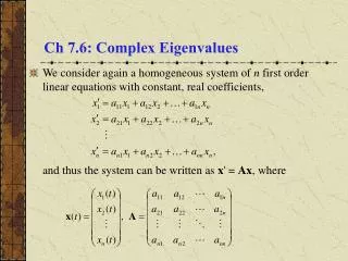
Ch 7.6: Complex Eigenvalues • We consider again a homogeneous system of n first order linear equations with constant, real coefficients, and thus the system can be written as x' = Ax, where
Conjugate Eigenvalues and Eigenvectors • We know thatx = ert is a solution of x' = Ax, provided r is an eigenvalue and is an eigenvector of A. • The eigenvalues r1,…, rnare the roots of det(A-rI) = 0, and the corresponding eigenvectors satisfy (A-rI) = 0. • If A is real, then the coefficients in the polynomial equation det(A-rI) = 0 are real, and hence any complex eigenvalues must occur in conjugate pairs. Thus if r1 = + i is an eigenvalue, then so is r2 = - i. • The corresponding eigenvectors (1), (2)are conjugates also. To see this, recall A and I have real entries, and hence
Conjugate Solutions • It follows from the previous slide that the solutions corresponding to these eigenvalues and eigenvectors are conjugates conjugates as well, since
Real-Valued Solutions • Thus for complex conjugate eigenvalues r1 and r2 ,the corresponding solutions x(1)and x(2)are conjugates also. • To obtain real-valued solutions, use real and imaginary parts of either x(1)or x(2). To see this, let (1) = a + ib. Then where are real valued solutions of x' = Ax, and can be shown to be linearly independent.
General Solution • To summarize, suppose r1 = + i, r2 = - i, and that r3,…, rnare all real and distinct eigenvalues of A. Let the corresponding eigenvectors be • Then the general solution of x' = Ax is where
Example 1: Direction Field (1 of 7) • Consider the homogeneous equation x' = Ax below. • A direction field for this system is given below. • Substituting x = ert in for x, and rewriting system as (A-rI) = 0, we obtain
Example 1: Complex Eigenvalues (2 of 7) • We determine r by solving det(A-rI) = 0. Now • Thus • Therefore the eigenvalues are r1= -1/2 + i and r2= -1/2 - i.
Example 1: First Eigenvector (3 of 7) • Eigenvector for r1= -1/2 + i: Solve by row reducing the augmented matrix: • Thus
Example 1: Second Eigenvector (4 of 7) • Eigenvector for r1= -1/2 - i: Solve by row reducing the augmented matrix: • Thus
Example 1: General Solution (5 of 7) • The corresponding solutions x = ert of x' = Ax are • The Wronskian of these two solutions is • Thus u(t)and v(t)are real-valued fundamental solutions of x' = Ax, with general solution x = c1u + c2v.
Example 1: Phase Plane (6 of 7) • Given below is the phase plane plot for solutions x, with • Each solution trajectory approaches origin along a spiral path as t , since coordinates are products of decaying exponential and sine or cosine factors. • The graph of u passes through (1,0), since u(0) = (1,0). Similarly, the graph of v passes through (0,1). • The origin is a spiral point, and is asymptotically stable.
Example 1: Time Plots (7 of 7) • The general solution is x = c1u + c2v: • As an alternative to phase plane plots, we can graph x1 or x2 as a function of t. A few plots of x1 are given below, each one a decaying oscillation as t .
Spiral Points, Centers, Eigenvalues, and Trajectories • In previous example, general solution was • The origin was a spiral point, and was asymptotically stable. • If real part of complex eigenvalues is positive, then trajectories spiral away, unbounded, from origin, and hence origin would be an unstable spiral point. • If real part of complex eigenvalues is zero, then trajectories circle origin, neither approaching nor departing. Then origin is called a center and is stable, but not asymptotically stable. Trajectories periodic in time. • The direction of trajectory motion depends on entries in A.
Example 2: Second Order System with Parameter (1 of 2) • The system x' = Ax below contains a parameter . • Substituting x = ert in for x and rewriting system as (A-rI) = 0, we obtain • Next, solve for r in terms of :
Example 2: Eigenvalue Analysis (2 of 2) • The eigenvalues are given by the quadratic formula above. • For < -4, both eigenvalues are real and negative, and hence origin is asymptotically stable node. • For > 4, both eigenvalues are real and positive, and hence the origin is an unstable node. • For -4 < < 0, eigenvalues are complex with a negative real part, and hence origin is asymptotically stable spiral point. • For 0 < < 4, eigenvalues are complex with a positive real part, and the origin is an unstable spiral point. • For = 0, eigenvalues are purely imaginary, origin is a center. Trajectories closed curves about origin & periodic. • For = 4, eigenvalues real & equal, origin is a node (Ch 7.8)
Second Order Solution Behavior and Eigenvalues: Three Main Cases • For second order systems, the three main cases are: • Eigenvalues are real and have opposite signs; x = 0 is a saddle point. • Eigenvalues are real, distinct and have same sign; x = 0 is a node. • Eigenvalues are complex with nonzero real part; x = 0 a spiral point. • Other possibilities exist and occur as transitions between two of the cases listed above: • A zero eigenvalue occurs during transition between saddle point and node. Real and equal eigenvalues occur during transition between nodes and spiral points. Purely imaginary eigenvalues occur during a transition between asymptotically stable and unstable spiral points.