Download
1 / 84
840 likes | 1.05k Views
SMT Solvers (an extension of SAT). Kenneth Roe. Boolean Satisfiability (SAT). p 1. ⋁. ⋀. p 2. . ¬. . . . ⋀. ⋁. ⋁. p n. Is there an assignment to the p 1 , p 2 , …, p n variables such that evaluates to 1?. Satisfiability Modulo Theories . p 1. x = y. ⋁. ⋀.

E N D
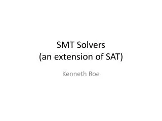
SMT Solvers(an extension of SAT) Kenneth Roe
Boolean Satisfiability (SAT) p1 ⋁ ⋀ p2 ¬ . . . ⋀ ⋁ ⋁ pn Is there an assignment to the p1, p2, …, pn variables such that evaluates to 1?
Satisfiability Modulo Theories p1 x= y ⋁ ⋀ p2 x + 2 z≥1 ¬ . . . ⋀ ⋁ w & 0xFFFF = x ⋁ x % 26 = v pn Is there an assignment to the x,y,z,w variables s.t. evaluates to 1?
Satisfiability Modulo Theories • Given a formula in first-order logic, with associated background theories, is the formula satisfiable? • Yes: return a satisfying solution • No [generate a proof of unsatisfiability]
Applications of SMT • Hardware verification at higher levels of abstraction (RTL and above) • Verification of analog/mixed-signal circuits • Verification of hybrid systems • Software model checking • Software testing • Security: Finding vulnerabilities, verifying electronic voting machines, … • Program synthesis • Scheduling
References Satisfiability Modulo Theories Clark Barrett, Roberto Sebastiani, Sanjit A. Seshia, and CesareTinelli. Chapter 8 in the Handbook of Satisfiability, Armin Biere, Hans van Maaren, and Toby Walsh, editors, IOS Press, 2009. (available from our webpages) SMTLIB: A repository for SMT formulas (common format) and tools (www.smtlib.org) SMTCOMP: An annual competition of SMT solvers
Roadmap for this Tutorial • Background and Notation • Survey of Theories • Equality of uninterpreted function symbols • Bit vector arithmetic • Linear arithmetic • Difference logic • Array theory • Combining theories • Review DLL • Extending DLL to DPLL(t)
Roadmap for this Tutorial • Background and Notation • Survey of Theories • Equality of uninterpreted function symbols • Bit vector arithmetic • Linear arithmetic • Difference logic • Array theory • Combining theories • Review DLL • Extending DLL to DPLL(t)
First-Order Logic • A formal notation for mathematics, with expressions involving • Propositional symbols • Predicates • Functions and constant symbols • Quantifiers • In contrast, propositional (Boolean) logic only involves propositional symbols and operators
First-Order Logic: Syntax • As with propositional logic, expressions in first-order logic are made up of sequences of symbols. • Symbols are divided into logical symbolsand non-logical symbols or parameters. • Example: (x = y) ⋀(y = z) ⋀(f(z) ➝f(x)+1)
First-Order Logic: Syntax • Logical Symbols • Propositional connectives: ⋀, ⋁, ¬, →,… • Variables: v1, v2, . . . • Quantifiers: 8, 9 • Non-logical symbols/Parameters • Equality: = • Functions: +, -, %, bit-wise &, f(), concat, … • Predicates: ·, is_substring, … • Constant symbols: 0, 1.0, null, …
Quantifier-free Subset • We will largely restrict ourselves to formulas without quantifiers (∀, ∃) • This is called the quantifier-free subset/fragment of first-order logic with the relevant theory
Logical Theory • Defines a set of parameters (non-logical symbols) and their meanings • This definition is called a signature. • Example of a signature: Theory of linear arithmetic over integers Signature is (0,1,+,-,·) interpreted over Z
Roadmap for this Tutorial • Background and Notation • Survey of Theories • Equality of uninterpreted function symbols • Bit vector arithmetic • Linear arithmetic • Difference logic • Array theory • Review DLL • Extending DLL to DPLL(t) • Combining theories
Some Useful Theories • Equality (with uninterpreted functions) • Linear arithmetic (over Q or Z) • Difference logic (over Q or Z) • Finite-precision bit-vectors • integer or floating-point • Arrays / memories • Misc.: Non-linear arithmetic, strings, inductive datatypes (e.g. lists), sets, …
Decision procedure • For each theory there is a decision procedure • Given a set of predicates in the theory, the procedure will always tell you whether or not they can be satisfied
Theory of Equality and Uninterpreted Functions (EUF) • Also called the “free theory” • Because function symbols can take any meaning • Only property required is congruence: that these symbols map identical arguments to identical values i.e., x = y ⇒f(x) = f(y) • SMTLIB name: QF_UF
x0 x1 x x2 ALU xn-1 Bit-vectors to Abstract Domain (e.g. Z) f Functional units to Uninterpreted Functions a = x ⋀b = y ⇒f(a,b) = f(x,y) Data and Function Abstraction with EUF Common Operations … p x 1 0 ITE(p, x, y) y If-then-else x = x = y y Test for equality
IF/ID ID/EX EX/WB PC Control Control Op Instr Mem Rd Ra = Adat Reg. File ALU Imm +4 = Rb Hardware Abstraction with EUF • For any Block that Transforms or Evaluates Data: • Replace with generic, unspecified function • Also view instruction memory as function F1 F2 F3
Example QF_UF (EUF) Formula (x = y) ⋀(y = z) ⋀(f(x) f(z)) Transitivity: (x = y) ⋀(y = z) →(x = z) Congruence: (x = z) →(f(x) = f(z))
Equivalence Checking of Program Fragments int fun1(int y) { int x, z; z = y; y = x; x = z; return x*x; } SMT formula Satisfiableiff programs non-equivalent ( z = y ⋀y1 = x ⋀x1 = z ⋀ret1 = x1*x1) ⋀ ( ret2 = y*y ) ⋀ ( ret1 ret2 ) int fun2(int y) { return y*y; } What if we use SAT to check equivalence?
Equivalence Checking of Program Fragments SMT formula Satisfiable iff programs non-equivalent ( z = y Æ y1 = x Æ x1 = z Æ ret1 = x1*x1) Æ ( ret2 = y*y ) Æ ( ret1 ret2 ) int fun1(int y) { int x, z; z = y; y = x; x = z; return x*x; } Using SAT to check equivalence (w/ Minisat) 32 bits for y: Did not finish in over 5 hours 16 bits for y: 37 sec. 8 bits for y: 0.5 sec. int fun2(int y) { return y*y; }
Equivalence Checking of Program Fragments int fun1(int y) { int x, z; z = y; y = x; x = z; return x*x; } SMT formula ’ ( z = y ⋀y1 = x ⋀x1 = z ⋀ret1 = sq(x1) ) ⋀ ( ret2 = sq(y) ) ⋀ ( ret1 ret2 ) int fun2(int y) { return y*y; } Using EUF solver: 0.01 sec
Equivalence Checking of Program Fragments int fun1(int y) { int x; x = x ^ y; y = x ^ y; x = x ^ y; return x*x; } Does EUF still work? No! Must reason about bit-wise XOR. Need a solver for bit-vector arithmetic. Solvable in less than a sec. with a current bit-vector solver. int fun2(int y) { return y*y; }
Finite-Precision Bit-Vector Arithmetic (QF_BV) • Fixed width data words • Can model int, short, long, etc. • Arithmetic operations • E.g., add/subtract/multiply/divide & comparisons • Two’s complement and unsigned operations • Bit-wise logical operations • E.g., and/or/xor, shift/extract and equality • Boolean connectives
Linear Arithmetic (QF_LRA, QF_LIA) • Boolean combination of linear constraints of the form (a1 x1 + a2 x2 + … + an xn» b) • xi’s could be in Q or Z , »2 {¸,>,·,<,=} • Many applications, including: • Verification of analog circuits • Software verification, e.g., of array bounds
Difference Logic (QF_IDL, QF_RDL) • Boolean combination of linear constraints of the form xi-xj» cijor xi»ci »2 {¸,>,·,<,=}, xi’s in Q or Z • Applications: • Software verification (most linear constraints are of this form) • Processor datapath verification • Job shop scheduling / real-time systems • Timing verification for circuits
Arrays/Memories • SMT solvers can also be very effective in modeling data structures in software and hardware • Arrays in programs • Memories in hardware designs: e.g. instruction and data memories, CAMs, etc.
Theory of Arrays (QF_AX)Select and Store • Two interpreted functions: select and store • select(A,i) Read from A at index i • store(A,i,d) Write d to A at index i • Two main axioms: • select(store(A,i,d), i) = d • select(store(A,i,d), j) = select(A,j) for i j • One other axiom: • (∀i. select(A,i) = select(B,i)) ) A = B
Equivalence Checking of Program Fragments int fun1(int y) { int x[2]; x[0] = y; y = x[1]; x[1] = x[0]; return x[1]*x[1]; } SMT formula ’’ [ x1 = store(x,0,y)Æ y1 = select(x1,1) Æ x2 = store(x1,1,select(x1,0)) Æ ret1 = sq(select(x2,1)) ] Æ ( ret2 = sq(y) ) Æ ( ret1 ret2 ) int fun2(int y) { return y*y; }
Roadmap for this Tutorial • Background and Notation • Survey of Theories • Equality of uninterpreted function symbols • Bit vector arithmetic • Linear arithmetic • Difference logic • Array theory • Combining theories • Review DLL • Extending DLL to DPLL(t)
Combining Theory Solvers • Theory solvers become much more useful if they can be used together. mux_sel = 0 → mux_out = select(regfile, addr) mux_sel = 1 → mux_out = ALU(alu0, alu1) • For such formulas, we are interested in satisfiability with respect to a combination of theories. • Fortunately, there exist methods for combining theory solvers. • The standard technique for this is the Nelson-Oppen method [NO79, TH96]. Slide taken from [Barret09 and Haney]
The Nelson-Oppen Method • Suppose that T1 and T2 are theories and that Sat 1 is a theory solver for T1-satisfiabilityand Sat 2 for T2-satisfiability. • We wish to determine ifφ is T1∪T2-satisfiable. • Convert φ to its separate form φ1 ∧ φ2. • Let S be the set of variables shared between φ1 and φ2. • For each arrangement D of S: • Run Sat 1 on φ1 ∪ D . • Run Sat 2 on φ2 ∪ D. Slide taken from [Barret09 and Haney]
Combining Theories • QF_UFLIA φ =1 ≤ x ∧ x ≤ 2 ∧ f(x) ≠ f(1) ∧ f(x) ≠ f(2) • We first convert φ to a separate form: • φUF = f(x) ≠ f(y) ∧ f(x) ≠ f(z) • φLIA = 1 ≤ x ∧ x ≤ 2 ∧ y = 1 ∧ z = 2 Slide taken from [Barret09 and Haney]
Φ IS UNSAT Combining Theories • φUF = f(x) ≠ f(y) ∧ f(x) ≠ f(z) • φLIA = 1 ≤ x ∧ x ≤ 2 ∧ y = 1 ∧ z = 2 • {x, y, z} can have 5 possible arrangements based on equivalence classes of x, y, and z • Assume All Variables Equal: • {x = y, x = z, y = z}inconsistent with φUF • Assume Two Variables Equal, One Different • {x = y, x ≠ z, y ≠ z}inconsistent with φUF • {x ≠ y, x = z, y ≠ z}inconsistent with φUF • {x ≠ y, x ≠ z, y = z}inconsistent with φLIA • Assume All Variables Different: • {x ≠ y, x ≠ z, y ≠ z}inconsistent with φLIA Slide adopted from [Barret09 and Haney]
Convex theories • Definition: Γ⊨T ⋁i∈Ixi =yiiff Γ⊨T xi =yi for some i∈I • Gives much faster combination • O(2n*n×(T1(n)+T2(n)) if one or both theories not convex • O(n3 × (T1(n) + T2(n))) if both are convex • Non-convex theories: • bit vector theories • linear integer arithmetic • theory of arrays
Stably infinite theories • A theory is stably infinite if every satisfiable QFF is satisfiable in an infinite model (Leonardo de Moura) • T2 =DC(∀x,y,z.(x=y)∨(x=z)∨(y=z))
Roadmap for this Tutorial • Background and Notation • Survey of Theories • Equality of uninterpreted function symbols • Bit vector arithmetic • Linear arithmetic • Difference logic • Array theory • Combining theories • Review DLL • Extending DLL to DPLL(t)
Basic DLL Procedure (a’ + b + c) (a + c + d) (a + c + d’) (a + c’ + d) (a + c’ + d’) (b’ + c’ + d) (a’ + b + c’) (a’ + b’ + c) 600.325/425 Declarative Methods - J. Eisner slide thanks to Sharad Malik (modified)
Basic DLL Procedure a (a’ + b + c) (a + c + d) (a + c + d’) (a + c’ + d) (a + c’ + d’) (b’ + c’ + d) (a’ + b + c’) (a’ + b’ + c) 600.325/425 Declarative Methods - J. Eisner slide thanks to Sharad Malik (modified)
Basic DLL Procedure Green means “crossed out” a (a’ + b + c) 0 Decision (a + c + d) a + (a + c + d’) a + (a + c’ + d) a + (a + c’ + d’) a + (b’ + c’ + d) (a’ + b + c’) (a’ + b’ + c) 600.325/425 Declarative Methods - J. Eisner slide thanks to Sharad Malik (modified)
Basic DLL Procedure a (a’ + b + c) 0 (a + c + d) a + (a + c + d’) b a + (a + c’ + d) a + 0 Decision (a + c’ + d’) a + (b’ + c’ + d) (a’ + b + c’) (a’ + b’ + c) 600.325/425 Declarative Methods - J. Eisner slide thanks to Sharad Malik (modified)
Basic DLL Procedure a (a’ + b + c) 0 (a + c + d) a + c + (a + c + d’) b a + c + (a + c’ + d) a + 0 (a + c’ + d’) a + c (b’ + c’ + d) (a’ + b + c’) 0 Decision (a’ + b’ + c) 600.325/425 Declarative Methods - J. Eisner slide thanks to Sharad Malik (modified)
Implication Graph(shows that the problem was caused by a=0 ^ c=0;nothing to do with b) (a + c + d) a=0 d=1 Conflict! c=0 d=0 (a + c + d’) Basic DLL Procedure a (a’ + b + c) 0 (a + c + d) a + c + Unit clauses force both d=1 and d=0: contradiction (a + c + d’) b a + c + (a + c’ + d) 0 (a + c’ + d’) c (b’ + c’ + d) (a’ + b + c’) 0 (a’ + b’ + c) 600.325/425 Declarative Methods - J. Eisner slide thanks to Sharad Malik (modified)
Basic DLL Procedure a (a’ + b + c) 0 (a + c + d) a + (a + c + d’) b a + (a + c’ + d) a + 0 (a + c’ + d’) a + c (b’ + c’ + d) Backtrack (a’ + b + c’) 0 (a’ + b’ + c) 600.325/425 Declarative Methods - J. Eisner slide thanks to Sharad Malik (modified)
Basic DLL Procedure a (a’ + b + c) 0 (a + c + d) (a + c + d’) b (a + c’ + d) a + c’ + 0 (a + c’ + d’) a + c’ + c (b’ + c’ + d) (a’ + b + c’) Other Decision 0 1 (a’ + b’ + c) (a + c’ + d) a=0 d=1 Conflict! c=1 d=0 (a + c’ + d’) 600.325/425 Declarative Methods - J. Eisner slide thanks to Sharad Malik (modified)
Basic DLL Procedure a (a’ + b + c) 0 (a + c + d) a + (a + c + d’) b Backtrack (2 levels) a + (a + c’ + d) a + 0 (a + c’ + d’) a + c (b’ + c’ + d) (a’ + b + c’) 0 1 (a’ + b’ + c) 600.325/425 Declarative Methods - J. Eisner slide thanks to Sharad Malik (modified)
Basic DLL Procedure a (a’ + b + c) 0 (a + c + d) a + (a + c + d’) b a + (a + c’ + d) a + Other Decision 0 1 (a + c’ + d’) a + c (b’ + c’ + d) b’ + (a’ + b + c’) 0 1 (a’ + b’ + c) 600.325/425 Declarative Methods - J. Eisner slide thanks to Sharad Malik (modified)
Basic DLL Procedure a (a’ + b + c) 0 (a + c + d) a + c + (a + c + d’) b a + c + (a + c’ + d) 0 1 (a + c’ + d’) c c (b’ + c’ + d) (a’ + b + c’) 0 0 1 Decision (a’ + b’ + c) (a + c’ + d) a=0 d=1 Conflict! c=0 d=0 (a + c’ + d’) 600.325/425 Declarative Methods - J. Eisner slide thanks to Sharad Malik (modified)
Basic DLL Procedure a (a’ + b + c) 0 (a + c + d) a + (a + c + d’) b a + (a + c’ + d) a + 0 1 (a + c’ + d’) a + c c Backtrack (b’ + c’ + d) b’ + (a’ + b + c’) 0 0 1 (a’ + b’ + c) 600.325/425 Declarative Methods - J. Eisner slide thanks to Sharad Malik (modified)
![SAT and CSP/CP Solvers [complete search]](https://cdn1.slideserve.com/1715685/slide1-dt.jpg)