Download
1 / 19
190 likes | 392 Views
SOLPS5 simulations of ELMing H-mode. Barbora Gulejov á Richard Pitts, David Coster, Xavier Bonnin, Roland Behn, Marc Beurskens, Stefan Jachmich, Jan HoráÄek, Arne Kallenbach. OUTLINE. SOLPS 5 code package ELM simulation - theory Simulation of Type III ELM at TCV

E N D
SOLPS5 simulations of ELMing H-mode Barbora Gulejová Richard Pitts,David Coster, Xavier Bonnin, Roland Behn, Marc Beurskens, Stefan Jachmich, Jan Horáček, Arne Kallenbach
OUTLINE SOLPS 5 code package ELM simulation - theory Simulation of Type III ELM at TCV Simulation of Type I ELMing H-mode at JET Code - experiment benchmark Code - code benchmark * * * * * *
MOTIVATION ELMing H-mode = baseline scenario for plasma operation on ITER! Edge localised mode (ELM) H-mode Edge MHD instabilities Periodic bursts of particles and energy into the SOL ELM leaves edge pedestal region in the form of a helical filamentary structure localised in the outboard midplane region of the poloidal cross-section Danger: divertor targets and main walls erosion first wall power deposition Energy stored in ELMs: TCV 500 J JET 200kJ ITER ~ 1-10 MJ => unacceptable Understanding of the ELM from formation to point of interaction with plasma facing components = Important research goal!
SOLPS5 modelling of ELMing H-mode *contribute to understanding transport in the SOL : transient events => ELMs * interpretative modeling of both 1.) steady state and 2.) transient particle and heat fluxes during ELMing H-mode employing the SOLPS5 fluid/Monte Carlo code * rigorous benchmarking = seeking the possible agreement between 1.) experiment and simulation 2.) code and different code MODEL: tool to understand and predict phenomena => 1.) • Type III & Type I ELMing H-mode • TCV & JET • benchmark SOLPS & EDGE2D/NIMBUS 2.a) 2.b)
Scrape-Off Layer Plasma Simulation Suite of codes to simulate transport in edge plasma of tokamaks B2 - solves 2D multi-species fluid equations on a grid given from magnetic equilibrium EIRENE - kinetic transport code for neutrals based on Monte - Carlo algorithm SOLPS 5 – coupled EIRENE + B2.5 Mesh plasma background => recycling fluxes 72 grid cells poloidally along separatrix 24 cells radially B2 EIRENE Sources and sinks due to neutrals and molecules Main inputs: * magnetic equilibrium * Psol = Pheat – Pradcore * upstream separatrix density ne *EELM Free parameters: cross-field transport coefficients (D┴, ┴, v┴) measured systematically adjusted D0 D1+ C0 C1+ C2+ C3+ C4+ C5+ C6+
Type III ELMing H-mode on TCV ELMs - too rapid (frequency ~ 200 Hz) for comparison on an individual ELM basis => Many similar events are coherently averaged inside interval with reasonably periodic elms telm ~ 100 μs tpost ~ 1 ms tpre ~ 2 ms Pre-ELM phase Post-ELM phase ELM = particles and heat are thrown into SOL ( elevated cross-field transport coefficients) Time-dependent ELM simulation * starting from time-dependent pre-ELM steady state simulation * equal time-steps for kinetic and fluid parts of code, dt = 10-6 s
Pre-ELM and ELM simulation - theory Cross-field radial transportin the main SOL - complex phenomena Ansatz:( D┴, ┴, v┴) – variation : radially – transport barrier (TB) poloidally – no TB in div.legs 2 approaches * Pure diffusion: v┴=0 everywhere * More appropriate: Convection simulations with D┴= D┴class Simulation of ELM Instantaneous increase of the cross-field transport parameters D┴, ┴, v┴! 1.) for ELM time – from experiment coh.averaged ELM = tELM = 10-4s 2.) at poloidal location -> expelled from area AELM at LFS Cross-field radial transport => approximate estimation of transport parameters during ELM corresponding to the given expelled energy WELM, tELM and AELM AELM= 1.5m2 W = 600 J 20 * D┴ ┴ 40 0 20
Type III TCV ELM simulation ELM is more convective than conductive ! Upstream TS measurements (R.Behn et al., PPCF 49 (2007)) => larger drop in ne than Te at the pedestal top => <Teped>Δ.nepedexceeds <neped>Δ.Teped in the contribution to EELM => SOLPS : D increased more then during the ELM 100times 10 times (2 times in SOL) + change of radial shape ! ETB collapse! AELM=1.5m2 – Gaussian function of multiplicators polloidally 1 ELM cycle of total 400 μs, * 100 μs before ELM * ELM duration = tELM = 100μs =100 points during ELM event * 200 μs after ELM smaller TB D┴ ┴ Very good agreement !
Type III TCV ELM simulation Downstream SOLPS < Exp (LP) factor ~ 1.5 SOLPS >> Exp (coav LP) ( R.Pitts,Nucl.Fusion 43 (2003)) factor ~ 3
Type I ELMing H-mode on JET Succesfully modelled by EDGE2D + NIMBUS by Arne Kallenbach (PPCF 46,2004) # 58569 Parameters Bt = 2 T Ip = 2 MA ne= 4x10¹⁹ m-3 P(SOL)= 12 MW GAS PUFF from inner divertor !! Dalpha PIN ~ 14 MW PRAD (core) ELM parameters felm ~ 30 Hz ΔWELM ~ 200 kJ Wdia CoreLIDAR Edge LIDAR Li beam ECE time
Benchmarking code-code SOLPS 5 B2.5 + EIRENE fluid (Braginskii) kinetic (Monte Carlo), neutrals vs. EDGE2D + NIMBUS fluid (Braginskii) kinetic (Monte Carlo), neutrals (less complex then EIRENE!)
Pre-ELM model vs.experiment EDGE2D+NIMBUS SOLPS5 2 2 Same Ansatz D,Chi,v Same ne,Te,Ti upstream profiles -0.05 0.05 0 r-rsep [m]
Pre-ELM vs. ELM simulation EDGE2D+NIMBUS SOLPS5 ELM D x 20 Chi x 40 1ms 0.05 -0.05 0.05 0 0.05 0.05 -0.05 0 0.1
Model vs. experiment-targets(LP) outer target inner target outer target EDGE2D+NIMBUS SOLPS5 250 300 LP 25 25 5 7 r-rsep map2mid r-rsep map2mid
Type I ELMing H-mode on JET =baseline scenario for QDT=10 burning plasma operation on ITER !!! To avoid divertor damage => maximum ΔWELM (ITER) ~ 1MJ(at TCV 0.005 MJ !!!) = this is achievable on JET # 70224 Parameters Bt = 3 T Ip = 3 MA ne=6x10¹⁹ m-3 P(SOL)= 19 MW No GAS PUFF !! ν*ped ~0.03 -0.08 (expected for ITER!) CoreLIDAR Edge LIDAR Li beam HRTS ECE Dalpha PIN ~ 20 MW PRAD(below Xpoint) PRAD (core) ELM parameters felm ~ 2 Hz ΔWELM ~ 1 MJ Langmuir probes Wdia Bolometry (A.Huber) radiation between ELMs Simulated for the first time ! … with SOLPS5 time
Simulation vs. experiment - upstream ne [m-3] First results for pre-ELM Te [eV] D┴= 0.01 m2.s-1 in pedestal 1 m2.s-1 in SOL Χ┴= 0.7 m2.s-1 in pedestal 1 m2.s-1 in SOL (TCV pedestal: D┴= 0.007 m2.s-1 Χ┴= 0.25 m2.s-1 ) D[m2.s-1] Χ[m2.s-1] CoreLIDAR Edge LIDAR Li beam HRTS ECE * quite promising * unlike for TCV inward pinch radial profile necessary!! vperp [m.s-1] inward pinch!
Simulation vs.experiment - targets SOLPS LP Inner target Outer target LP 80 50 50 30 1,2 0.5 r-rsep r-rsep r-rsep map2mid r-rsep map2mid Inner target – good agreement Outer target SOLPS Te too high!
CONCLUSIONS Type III ELMing H-mode at TCV and Type I ELMing H-mode at JET have been succesfully simulated by SOLPS5 both steady state and transient event Agreement obtained between : code - experiment code - code * * * * * *