Download
1 / 66
730 likes | 1.12k Views
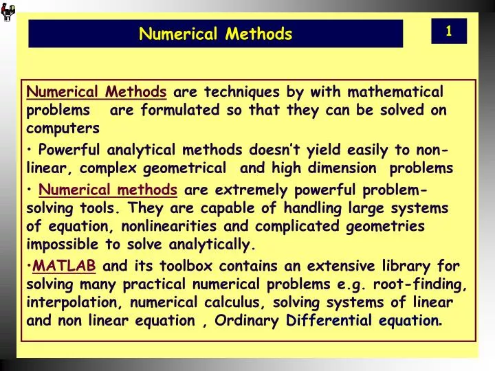
Numerical Methods. Numerical Methods are techniques by with mathematical problems are formulated so that they can be solved on computers Powerful analytical methods doesn’t yield easily to non-linear, complex geometrical and high dimension problems

E N D
Numerical Methods Numerical Methods are techniques by with mathematical problems are formulated so that they can be solved on computers Powerful analytical methods doesn’t yield easily to non-linear, complex geometrical and high dimension problems Numerical methods are extremely powerful problem-solving tools. They are capable of handling large systems of equation, nonlinearities and complicated geometries impossible to solve analytically. MATLAB and its toolbox contains an extensive library for solving many practical numerical problems e.g. root-finding, interpolation, numerical calculus, solving systems of linear and non linear equation , OrdinaryDifferential equation.
Numerical Methods • Contents • Solving linear equation of system • Matrix Factorization/Decomposition Techniques • Curve fitting and polynomials operations • Interpolation • Numerical Integration and Differentiation • Ordinary Differential Equation • Non-linear equations
Linear Algebra • Solving a linear system 5x = 3y - 2z + 10 8y + 4z = 3x +20 2x + 4y - 9z = 9 • Cast in standard matrix form A x = b
Linear Equations A = [5 -3 2; -3 8 4; 2 4 -9]; b = [10; 20; 9]; Left Division Method x = A \ b • Check solution c = A*x • c should be equal to b.
Gaussian Elimination • Pivoting C = [ A b] % augmented matrix • row reduced echelon form Cr = rref(C) Cr = 1.0000 0 0 3.4442 0 1.0000 0 3.1982 0 0 1.0000 1.1868
Eigenvalues and Eigenvectors • The problem A v = v • With pencil-paper, we must solve for det (A - ) = 0 then solve the linear equation • MATLAB way [V, D] = eig(A) [V,D] = EIG(X) produces a diagonal matrix D of eigenvalues and a full matrix V whose columns are the corresponding eigenvectors so that X*V = V*D.
Matrix Factorizations • LU decomposition [L, U] = lu(A) such that L*U = A, L is a lower triangular matrix, U is an upper triangular matrix. • DSP blockset (Simulink)
Matrix Factorization • QR factorization – Application in Curve fitting, [Q, R] = qr(A) %m>n – over determined If n=rank(A) then A[Q,R] Anxn such that Q*R = A; Q is orthogonal matrix ,independent row/coloums and R is upper triangular matrix. QT=Q-1, QT*Q=I • DSP blockset (Simulink)
Matrix factorization • Singular Value Decomposition [U, D, V] = svd(A) such that UDV = A, where U and V are orthogonal and D is diagonal matrix [Eigen values]. • DSP Blockset A = [1 1 1; 2 -1 2; -1 4 3; 4 2 1; 3 -3 4] b = [1; 2; -1; 4; 8] S = svd(A); [U,S,V] = svd(A); U*S*V'
Sparse Matrix • See help sparfun for detail The sparse function generates matrices in the MATLAB sparse storage organization. S = sparse(A) converts a full matrix to sparse form by squeezing out any zero elements. If S is already sparse, sparse(S) returns S. A=[1 0 1; 0 2 0; 3 3 0]; S=sparse(A); is =[1 3 2 3 1],js =[1 1 2 2 3],as =[1 3 2 3 1]; S=sparse(is,js,as) %Tabular..
Curve Fitting – Polyfit & Polyval- • Polynomial curve fitting • a=polyfit(x,y,n) • do a least-square fit with polynomial of degree n. x and y are data vectors, and a is coefficients of the polynomial, a = [an, an-1, …, a1, a0] • Store data and perform the fit • x =[1 2 4 5 ]; %data • y =[1 2 2 3 ]; %data • c =polyfit(x,y,n) %n=1 degree • Evaluate and plot the fit with • xfit=[0 6] • yfit =c(1)*xfit +c(2) %y=c(1)x + c(2) • plot(x,y,’o ’,xfit,yfit,’-’); • grid
Curve Fitting- Non Linear Functions • y = polyval(a, x) • compute the value of polynomial at value x y = a(1) x^n + a(2) x^(n-1) + … + a(n) x + a(n+1) • The Polynomial is evaluated at x=5, 7, and 9 with p = [3 2 1]; polyval(p,[5, 7, 9]) CURVE FITTING TOOLBOX
Curve Fitting- Least Square Fit Normal Equations Consider the problem Axb, where A is an (m,n) matrix with mn , rank(A) = n, b is an (m,1) vector, and x is the (n,1) vector, to be over determined. More equation than unknowns. In such case exact solution is not obtained Ax=b b c Least square provides the solution such that=
Normal Equation Least Square curve Fit Fit [x,y] data to x=[ 0.955 1.380 1.854 2.093 2.674 3.006 3.225 3.940 4.060]’; y=[5.722 4.812 4.727 4.850 5.011 5.253 5.617 6.2282 6.255]’; A=[1./x x]; %Coefficients matrix of overdetermined system c=(A’*A)\(A’*y); %Solve Normal equation xf= linspace(min(x), max(x)); yf=c(1)./xf + c(2)*xf Af=[1./xf’ xf’] yf=Af*c; plot(x, y,‘o’,xf, yf,‘-’); grid
z x y Curve Fit – Multivariate Least Square • Fitting Data to a plane • The equation can be solve for c’s as overdetermined m>n A * c = Z c = Z/A
Curve Fit – Multivariate Least Square clf x=[-4:1:4]' y=[4 -3 5 -4 1 -3 4 -1 3]' z=[18.74 -1.10 19.88 -5.71 6.20 -10.37 4.96 -5.30 1.54]' A=[x y ones(size(x))] c=A\z xg=linspace(-5,5,10); yg=xg; [X,Y]=meshgrid(xg,yg); Z=c(1)*X+c(2)*Y+c(3); plot3(x,y,z,'k.') hold surf(X,Y,Z) grid hold off
Polynomials • Polynomials are widely used in engineering… • How does Matlab represent a polynomial: • How can we use this? p=[1 3 -6 -2 7 -12]; p p = 1 3 -6 -2 7 -12 polyval(p,1) ans = -9 polyval(p,-1) ans = -13 polyval(p,3.32) ans = 537.4667 polyval(p,0) ans = -12
Polynomial Operations • There are a number of things we might like to do with polynomials: • find roots:roots(p) • reconstruct from roots:poly(p) • multiplication:conv(p1,p2) • division:[q,r]=deconv(pnum,pdenom) • addition or subtraction:you’re on your own! • derivative:polyder(p) • rational:we’ll leave this for an advanced class! • curvefitting:polyfit(x,y,ndeg)
Types of Interpolation • Interpolation involves computing approximate values between limiting or endpoint values • constant (zeroth order, nearest neighbor) • linear • cubic • spline • Equivalent to what is often called “table lookup” • Matlabyi=interp1(x,y,xi,’method’ )function: • x,yare vectors defining the “table of values” • xiis the independent variable • yiis the interpolated result • ‘method’is: linear (default), nearest, cubic, spline • this function can treat xi,yias vectors
Interpolation • This example compares different interpolation methods for 6 points defining a sine function echo on hold off clf x=linspace(0,2*pi,6); y=sin(x); plot(x,y,'or') hold on pause xi=linspace(0,2*pi,100); yi=interp1(x,y,xi,'nearest'); plot(xi,yi) pause yi2=interp1(x,y,xi); plot(xi,yi2,'g') pause yi3=interp1(x,y,xi,'cubic'); plot(xi,yi3,'k') pause yi4=interp1(x,y,xi,'spline'); plot(xi,yi4,'c') pause plot(xi,sin(xi),'r:') legend('data','nearest','linear','cubic','spline','sine') xlabel('X'), ylabel('Y')
2D Interpolation: interp2() • A bivariate function z-sin(x2+y2) is interpolated on the square -1x 1, -1y 1 using ‘linear’ and ‘cubic’ methods [x,y]=meshgrid(-1: 0.25:1); z=sin(x.^2 + y.^2); [xi, yi]=meshgrid(-1:0.05:1); zi=interp2(x,y,z,xi,yi,’linear’) surf(xi, yi, zi),title(‘Bilinear-interpolant to sin(x^2+y^2)’) zi=interp2(x,y,z,xi,yi,’cubic’) surf(xi, yi, zi),title(‘Bicubic-interpolant to sin(x^2+y^2)’)
Numerical Differentiation .Backward Difference .Forward Difference .Average of mA and mB .diff()function Central Diff. x=[0:pi/50:pi]; n=length(x); td=cos(x); y=sin(x)- 0.05*(rand(1,51)-0.5); d1=diff(y)./diff(x); %Backward Diff. subplot(2,1,1), plot(x(2:n), td(2:n),x(2:n),d1,’o’) xlabel(‘x’), ylabel(‘Derivative’) axis([0 pi –2 2]) ; d2=(y(3:n)-y(1:n-2))./(x(3:n)-x(1:n-2)); subplot(2,1,2), plot(x(2:n-1), td(2:n-1),x(2:n-1), d2,’o’),xlabel(‘x’),ylabel(‘Derivative’), axis([0 pi –2 2]),title(‘Central Diff.’),grid
Numerical methods for Root finding • Numerical methods are recipes that allow us to solve generic problems, e.g. Root finding • Bisection, false position, secant method, Newton’s Method • To use these method’s effectively requires we • Have a basis for comparing between alternatives • Know when each will and won’t work and why • Study of numerical methods involves • Development of algorithms • Study of their properties, e.g. convergence, stability, etc.
Recap - Newton’s method • The iteration formula for Newton’s method is • Can think of Newton’s method as a fixed point iteration scheme with • The derivative of g(x) is • Hence for Newton’s Method to converge
This term approximates the inverse of the gradient. Secant method…Roots Generalform of iteration equation
Secant method ….Roots Point: The secant method can be interpreted as Newton’s method with an approximated gradient.
Differential Equations Ordinary differential equations (ODE’s) arise in almost every field ODE’s describe a function y in terms of its derivatives The goal is to solve for y
Numerical Solution to ODEs In general, only simple (linear) ODEs can be solved analytically Most interesting ODEs are nonlinear, must solve numerically The idea is to approximate the derivatives by subtraction
Matlab’s ODE solvers Matlab has several ODE solvers: ode23 and ode45 are “standard” RK solvers ode15s and ode23s are specialized for “stiff” problems several others, check help ode23 or book
Simplest ODE scheme, but not very good “1st order, explicit, multi-step solver” General multi-step solvers: Euler Method (weighted mean of f evaluated at lots of t’s)
Runge-Kutta Methods Multi-step solvers--each N is computed from N at several times can store previous N’s, so only one evaluation of f/iteration Runge-Kutta Methods: multiple evaluations of f/iteration:
Example: differential equation General ODE: This example is model of an electronic circuit with a nonlinear vacuum tube, called van den Pol equation.
Example: differential equation • Construct an m-file function for the right-hand side of fvdp.m function dxdt = fvdp(t,x) % dxdt = fvdp(t,x) % van der Pol equation dxdt =[x(2,:); ... (1-x(1,:).^2).*x(2,:)-x(1,:)] ; Solve the ODE in the time span 0<t<10 [t,x] = ode45(’fvdp’,[0,10],[2;0]); plot(t,x) plot(x(:,1),x(:,2))
OPTIONAL MATERIAL: Solving ODE’s • Matlab includes a number of functions to solve Ordinary Differential Equations (ODE’s), including Initial Value Problems (IVP’s), Boundary Value Problems (BVP’s) and Partial Differential Equations (PDE’) • Let’s consider a simple IVP in the form of a familiar ODE (an sdof vibration problem): • Matlab’s ode23() and ode(45) functions use the Runge-Kutta-Fehlberg method to solve ODE’s expressed as: This is advanced material you will cover in your next math classes. Matlab will be there when you need it!
Solving an ODE: setup • We can convert an Nth order ODE into N first order ODE’s using a simple algorithm: • In more compact forms: or
Matlabode45( )Syntax >> help ode45 ODE45 Solve non-stiff differential equations, medium order method.[T,Y] = ODE45(ODEFUN,TSPAN,Y0) with TSPAN = [T0 TFINAL] integrates the system of differential equations y' = f(t,y) from time T0 to TFINAL with initial conditions Y0. Function ODEFUN(T,Y) must return a column vector corresponding to f(t,y). Each row in the solution array Y corresponds to a time returned in the column vector T. To obtain solutions at specific times T0,T1,...,TFINAL (all increasing or all decreasing), use TSPAN = [T0 T1 ... TFINAL]. (truncated) • [T,Y] are the returned values and each row defines a value of t where the solution is computed along with the corresponding solutions, yi , in successive columns. • But we need to provide a function to compute f(t,y) wheneverode45( )needs it… • We also need to specify the start and end times and initial conditions in the arguments toode45( )
rhs( )function forode45( ) • m-function will compute f(t,y) for ode45( ) • returns the RHS column vector NOTE:If you need to pass parameter values to compute the RHS (e.g, zeta or g(t)), these can be added to theode45( )function call (see help ode45)
Solving the Problem… Seehelp ode45for more options >> [tt,yy]=ode45('rhs', [0 35],[1 0]'); >> whos Name Size Bytes Class tt 205x1 1640 double array yy 205x2 3280 double array Grand total is 615 elements using 4920 bytes >> plot(tt,yy(:,1)) • Note the sizes of the returned variables • You can plot either column of yy as needed • How would you construct a phase plane plot (e.g., y versus y’)? You supply this m-function…
A More Interesting RHS… Note how g(t) is formed here Result is familiar square pulse with ringing oscillations
Simulink Example Best thing to do is to go through an example 2nd order, constant coefficient, linear differential equation Response to a “step” command
Simulink Example Get an equivalent block diagram for the system use mouse to drag blocks into the model window and to connect blocks with arrows use integrators to get dy/dt and y