Download

1 / 21
220 likes | 240 Views
Understand linear relationships using least-squares method. Examples on electrical currents and potential differences. Learn about measuring uncertainties and fitting procedures.

E N D
CHAPTER 6 LEAST-SQUARES FIT TO A STRAIGHT LINE
6.1 DEPENDENT AND INDEPENDENT VARIABLES We often wish to determine one characteristic y of an experiment as a function of some other quantity x. That is, instead of making a number of measurements of a single quantity x, we make a series of N measurements of the pair (Xi> yJ, one for each of several values of the index i, which runs from 1 to N. Our object is to find a function y = y(x) that describes the relation between these two measured variables. In this chapter we consider the problem of pairs of variables (x;, yJ that are linearly related to one another, and refer to data from two undergraduate laboratory experiments as examples. In the following chapters, we shall discuss methods of finding relationships that are not linear. 98 Example 6.1. A student is studying electrical currents and potential differences. He has been provided with a I-m nickel-silver wire mounted on a board, a lead-acid battery, and an analog voltmeter. He connects cells of the battery across the wire and measures the potential difference or voltage between the negative end and various positions along the wire. From examination of the meter, he estimates the uncertainty in each potential measurement to be 0.05 V. The uncertainty in the position of the probe is less than 1 mm and is considered to be negligible. The data are listed in Table 6.1 and are plotted in Figure 6.1 to show the potential difference as a function of wire length x. The estimated common uncertainty in each measured potential difference is indicated on the graph by the vertical error bars. From these measurements, we wish to find the linear function y(x) (shown as a solid line) that describes the way in which the voltage V varies as a function of position x along the wire.
We cannot fit a straight line to the data exactly in either example because it is impossible to draw a straight line through all the points. For a set of N arbitrary points, it is always possible to fit a polynomial of degree N - 1 exactly, but for our experiments, the coefficients of the higher-order terms would have questionable significance. We assume that the fluctuations of the individual points above and below the solid curves are caused by experimental uncertainties in the individual measurements. In Chapter 11 we shall develop a method for testing whether higherorder terms are significant. Measuring Uncertainties If we were to make a series of measurements of the dependent quantity Yi for one particular value Xi of the independent quantity, we would find that the measured values were distributed about a mean in the manner discussed in Chapter 5 with a probability of -68% that any single measurement of Yi be within 1 standard deviation of the mean. By making a number of measurements for each value of the independent quantity Xi' we could determine mean values Yi with any desired precision. Usually, however, we can make only one measurement Yi for each value of X = Xi' so that we must determine the value of Y corresponding to that value of X with an uncertainty that is characterized by the standard deviation (J'i of the distribution of data for that point.
We shall assume for simplicity in all the following discussions that we can ascribe all the uncertainty in each measurement to the dependent variable. This is equivalent to assuming that the precision of the determination of x is considerably higher than that of y. This difference is illustrated in Figures 6.1 and 6.2 by the fact that the uncertainties are indicated by error bars for the dependent variables but not for the independent variables. Our condition, that we neglect uncertainties in x and consider just the uncertainties in y, will be valid only if the uncertainties in Y that would be produced by variations in x corresponding to the uncertainties in the measurement of x are much smaller than the uncertainties in the measurement of y. This is equivalent, in first order, to the requirement at each measured point that dy (Jxdx q: (Jy where dy/dx is the slope of the function y = y(x). We are not always justified in ascribing all uncertainties to the dependent parameter. Sometimes the uncertainties in the determination of both quantities x and y are nearly equal. But our fitting procedure will still be fairly accurate if we estimate the indirect contribution (JyIfrom the uncertainty (Jx in x to the total uncertainty in y by the first-order relation (6.2) and combine this with the direct contribution (JyD' which is the measuring uncertainty in y, to get (6.3) For both Examples 6.1 and 6.2 the condition would be reasonable because we predict a linear dependence of y with x. With the linear assumption, we treat the uncertainties in our data as if they were in the dependent variable only, while realizing that the corresponding fluctuations may have been originally derived from uncertainties in the determinations of both dependent and independent variables. In those cases where the uncertainties in the determination of the independent quantity are considerably greater than those in the dependent quantity, it might be wise to interchange the definition of the two quantities.
6.2 METHOD OF LEAST SQUARES Our data consist of pairs of measurements (Xi' y) of an independent variable x and a dependent variable y. We wish to find values of the parameters a and b that minimize the discrepancy between the measured values Yi and calculated values y(x). We cannot determine the parameters exactly with only a finite number of observations, but can hope to extract the most probable estimates for the coefficients in the same way that we extracted the most probable estimate of the mean in Chapter 4. Before proceeding, we must define our criteria for minimizing the discrepancy between the measured and predicted values Yi' For any arbitrary values of a and b, we can calculate the deviations LlYibetween each of the observed values Yi and the corresponding calculated or fitted values LlYi= Yi- y(xJ= Yi- a - bXi (6.4) With well chosen parameters, these deviations should be relatively small. However, the sum of these deviations is not a good measure of how well our calculated straight line approximates the data because large positive deviations can be balanced by negative ones to yield a small sum even when the fit of the function y(x) to the data is bad. We might consider instead summing the absolute values of the deviations, but this leads to difficulties in obtaining an analytical solution. Instead we sum the squares of the deviations. There in no correct unique method for optimizing the parameters valid for all problems. There exists, however, a method that can be fairly well justified, that is simple and straightforward, 'and that is well established experimentally. This is the' method of least squares, similar to the method discussed in Chapter 4, but extended to include more than one variable. It may be considered as a special case of the more general method of maximum likelihood.
Method of Maximum Likelihood Our data consist of a sample of observations drawn from a parent distribution that determines the probability of making any particular observation. For the particular problem of an expected linear relationship between dependent and independent variables, we define parent parameters ao and bo such that the actual relationship between Y and x is given by (6.5) We shall assume that each individual measured value of Yi is itself drawn from a Gaussian distribution with mean Yo(x) and standard deviation (Ji' We should be aware that the Gaussian assumption may not always be exactly true. In Example 6.2 the Yi = Ci were obtained in a counting experiment and therefore follow a Poisson distribution. However, for a sufficiently large number of counts Yi the distribution may be considered to be Gaussian. We shall discuss fitting with Poisson statistics in Section 6.6. With the Gaussian assumption, the probability Pi for making the observed measurement Yi with standard deviation (Ji for the observations about the actual value Yo (Xi) is P 1 { 1 [Yi - YO(xJ]2} i = exp -- (Ji~ 2 (Ji (6.6) The probability for making the observed set of measurements of the N values of Yi is the product of the probabilities for each observation: () ( 1 ) {I ~ [Yi - YO(XJ P ao, bo = IIPi = II ]2} (Ji ~ exp -2: ~ (Ji (6.7)
where the product II is taken with iranging from I to N and the product of the exponentials has been expressed as the exponential of the sum of the arguments. In these products and sums, the quantities 1/a} act as weighting factors. Similarly, for any estimated values of the parameters a and b, we can calculate the probability of obtaining the observed set of measurements (6.8) with y(x) defined by Equation (6.1) and evaluated at each of the values Xi' We assume that the observed set of measurements is more likely to have come from the parent distribution of Equation (6.5) than from any other similar distribution with different coefficients and, therefore, the probability of Equation (6.7) is the maximum probability attainable with Equation (6.8). Thus, the maximumlikelihood estimates for a and b are those values that maximize the probability of Equation (6.8). Because the first factor in the product of Equation (6.8) is a constant, independent of the values of a and b, maximizing the probability pea, b) is equivalent to minimizing the sum in the exponential. We define this sum to be our goodness-offit parameter X2: (6.9) We use the same symbol X2, defined earlier in Equation (4.32), because this is essentially the same definition in a different context. Our method for finding the optimum fit to the data will be to find values of a and b that minimize this weighted sum of the squares of the deviations X2 and hence, to find the fit that produces the smallest sum of the squares or the leastsquares fit. The magnitude of X2 is determined by four factors: 1. Fluctuations in the measured values of the variables Yi' which are random samples from a parent population with expectation values Yo (x). 2. The values assigned to the uncertainties aiin the measured variables Yi' Incorrect assignment of the uncertainties a iwill lead to incorrect values of X2. 3. The selection of the analytical function y(x) as an approximation to the "true" function Yo(x). It might be necessary to fit several different functions in order to find the appropriate function for a particular set of data. 4. The values of the parameters of the function y(x). Our objective is to find the "best values" of these parameters.
6.3 MINIMIZING X2 To find the values of the parameters a and b that yield the minimum value for X2, we set to zero the partial derivatives of X2 with respect to each of the parameters Least-Squares Fit to a Straight Line 105 ~X2 = ~ ~r~(y. - a - bX)2] aa aalaT1 =-2~r~la (Ty .1 - a - bX1.) ] = 0 :b X2 = aab~[~T(Yi - a - bXY] (6.10) = -2~[~T(Yi - a - bxJ] = 0 These equations can be rearranged as a pair of linear simultaneous equations in the unknown parameters a and b: (6.11) The solutions can be found in anyone of a number of different ways, but, for generality we shall use the method of determinants. (See Appendix B.) The' solutions are ~lL ~;~ I a f a=- 1 1 = !(~ xT~ lL_ ~ ~ ~ XiYi) il ~XiYi ~;if2 il aT aT aT aT a f 1 1 1 ~ZL b=! ~-:z a2 ai=!(~~~XiYi_~ Xi ~lL) I il ~ Xi ~XiYi il aT aT aT aT a2 a2 1 1 (6.12) For the special case in which all the uncertainties are equal (a = ai), they cancel and the solutions may be written _ 1 ILYi LXi 1_ 1 ('" 2'" '" '" ) a - il' LX;)'i LXT - il' ,,:,Xi":'Yi - ,,:,Xi,,:,XiYi b = i1l' ILNX iLLXY;i )'iI= i1l' (NLxiYi- LXiLyJ(6.13) il' = IN LXi 1= NLxf - (Lx.)2 LXi LXY 1 1
Examples For the data of Example 6.1 (Table 6.1), we assume that the uncertainties in the measured voltages V are all equal and that the uncertainties in Xi are negligible. We can therefore use Equation (6.l3). We accumulate four sums LXi' LYi= LVi' LXI, and LXiYi= LXiViand combine them according to Equation (6.l3) to find numerical values for a and b. The steps of the calculation are illustrated in Table 6.1, and the resulting fit is shown as a solid line on Figure 6.1. Determination of the parameters a and b from Equation (6.12) is somewhat more tedious, because the uncertainties aimust be included. Table 6.2 shows steps in the calculation of the data of Example 6.2 with the uncertainties aiin the numbers of counts Ci determined by Poisson statistics so that aT= Ci• The values of a and b found in this calculation were used to calculate the straight line through the data points in Figure 6.2. It is important to note that the value of Ci to be used in determining the uncertainty a imust be the actual number of events observed. If, for example, the student had decided to improve her statistics by collecting data at the larger distances over longer time periods Lltiand to normalize all her data to a common time interval Lltc' C; = C; X LltclMi then the statistical uncertainty in C' would be given by a; = V""C; X MclMi Program 6.1. FITLI N E (Appendix E) Solution of Equations (6.11) by the determinant method of Equation (6.12). The program uses routines in the programs units FITVARS, FITUTI L, and G E NUT I L, which are also used by other fitting programs. The sample programs use single precision variables for simplicity, although double, or higher, precision is highly recommended. Program 6.1 uses Equation (6.12) to solve both Examples 6.1 and 6.2, although separate routines written for each problem would be slightly more efficient. Because the measurements of Example 6.1 have common errors, we could, for example, increase the fitting speed by using Equations (6.13) rather than Equations (6.12). Similarly, for Example 6.2, we could simplify the fitting routine by replacing the statistical errors SIGY[I] by the explicit expression for ~. However, in most calculations that involve statistical errors, there are also other errors to be considered, such as those arising from background subtractions, so the loss of generality would more than compensate for any increased efficiency in the calculations. Program 6.2. FITVARS (website) Include file of constants, variables, and arrays for least-squares fits. Program 6.3. FITUTI L (website) Utility routines for fitting programs Input/output routine, X2 calculation, x2-density, and x2-integral probability.
6.4 ERROR ESTIMATION Common Uncertainties If the standard deviations aifor the data points Yi are unknown but we can assume that they are all equal, aT= a2 , then we can estimate them from the data and the results of our fit. The requirement of equal errors may be satisfied if the uncertainties are instrumental and all the data are recorded with the same instrument and on the same scale, as was assumed in Example 6.1. In Chapter 2 we obtained, for our best estimate of the variance of the data, sample, 1 a2 = S2 == --2: (Yi- y)2 N-m (6.14) where N - m is the number of degrees of freedom and is equal to the number of measurements minus the number of parameters determined from the fit. In Equation (6.14) we identify Yi with the measured value of the dependent variable, and for y, the expected mean value of Yi' we use the value calculated from Equation (6.1) for each data point with the fitted parameters a and b. Thus, our estimate ai= a for the standard deviation of an individual measurement is a2 = S2 = N ~ 2 2: (Yi - a - bx Y (6.15) By comparing Equation (6.15) with Equation (6.9), we see that it is just this common uncertainty that we have minimized in the least-squares fitting procedure. Thus, we can obtain the common error in our measurements of Y from the fit, although at the expense of any information about the quality of the fit. Variable Uncertainties In general the uncertainties a iin the dependent variables Yi will not all be the same. If, for example, the quantity Y represents the number of counts in a detector per unit time interval (as in Example 6.2), then the errors are statistical and the uncertainty in each measurement Yi is directly related to the magnitude of Y (as discussed in Section 4.2), and the standard deviations aiassociated with these measurements is (6.16) In principle, the value of Yi' which should be used in calculating the standard deviations aiby Equation (6.16), is the value Yo(x;) of the parent population. In practice we use the measured values that are only samples from that population. In the limit of an infinite number of determinations, the average of all the measurements would very closely approximate the parent value, but generally we cannot make more than one measurement of each value of x, much less an infinite number. We
coul~ approximate the parent value Yo (x;) by using the calculated value y(x) from o~~ fIt, but th~t would complicate the fitting procedure. We shall discuss this possibIlIty further m the following section. Contributions from instrumental and other uncertainties may modify the simple square root form of the statistical errors. For example, uncertainties in measuring t~e time interval during which the events of Example 6.2 were recorded might contnbute, although statistical fluctuations generally dominate in counting experi~ ents. Ba.ckground subtractions are another source of uncertainty. In many countmg exp~nments, there .is a background under the data that may be removed by subtractIOn, or may be mcluded in the fit. In Example 6.2, cosmic rays and other backgrounds contrib~te ~o a counting rate even when the source is moved far away from the detecto:, as mdIcated by the nonzero intercept of the fitted line of Figure 6.2 on the C aXIS. If the student had chosen to record the radiation background counts Cbin a separate measurement and to subtract Cbfrom each of her measurements Ci to obtain C; = Ci - Cb then the uncertainty in C' would have been given by combining in quadrature the uncertainties in the two measurements: x2 Probability For those data for which we know the uncertainties <Tiin the measured values y. we can calculate the value of X2 from Equation (6.9) and test the goodness of ou; fit. For our two-parameter fit to a straight line, the number of degrees of freedom will be N - 2. Then, for the data of Example 6.2, we should hope to obtain X2 = 10 - 2 = 8. The actual value, X2 = 11.1, is listed in Table 6.2, along with the probability (p = 20%). (See Table C:.4.) We interpret this probability in the following way. Suppose that we have obtamed a X2 probability of p% for a certain set of data. Then, we should expect that, if we were to repeat the experiment many times, approximately p% of the experiments would yield X2 values as high as the one that we obtained or higher. This subject will be discussed further in Chapter 11. In Example 6.1, we obtained a value of X2 = 1.95 for 7 degrees of freedom, corres~on.ding to. a probability of about 96%. Although this probability may seem to be gratIfymglyhIgh, the very low value of X2 gives a strong indication that the common uncertainty in the data may have been overestimated and it might be wise to use th.e value of X2 to obtain a better estimate of the common uncertainty. From EquatIOns (6.15) and (6.9), we obtain an expression for the revised common uncertainty <T: in terms of X2 and the original estimate, <Tc: <T~2 = <Tf X X2/(N - 2) (6.17) or, more generally (6.18) where X~ = X21v and v is the number of degrees of freedom in the fit. Thus, for Example 6.1, we find <T?= 0.052 X 1.95/(9 - 2) = 0.0007, or <T: = ~0.03 V.
Uncertainties in the Parameters In order to find the uncertainty in the estimation of the parameters a and b in our fitting procedure, we use the error propagation method discussed in Chapter 3. Each of our data points Yi has been used in the determination of the parameters and each has contributed some fraction of its own uncertainty to the uncertainty in our final determination: Ignoring systematic errors, which would introduce correlations between uncertainties, the variance <T~ of the parameter z is given by Equation (3.14) as the sum of the squares of the products of the standard deviations <Tiof the data points with the effects that the data points have on the determination of z: (6.19) Thus, to determine the' uncertainties in the parameters a and b, we take the' partial derivatives of Equation (6.12): aa 1 ( 1 XfXj Xi) -=- -~---~- a YjLl<TJ <Tf<TJ <Tf (6.20) ab =~(Xj ~~_~~ Xi) a YjLl<TJ <Tf<TJ <Tf We note that the derivatives are functions only of the variances and of the independent variables Xi. Combining these equations with the general expression of Equation (6.19) and squaring, we obtain for <T2, <T~ = ~ <T~ [~ (~X~)2 _ 2; ~ X~ ~ x~ + X~ (~ X~)2] j=! Ll <Tj<Ti<Tj<Ti <Ti<Tj<Ti = ~2 [~:2(~ ;~)2_ 2~;~ ~ ;~~ ;~ + ~ ~ (~;~)2] J I J I I J I = ~2(~;~)[~:J~;~-(~;f)2] =i~;~ I (6.21) (6.22)
For the special case of common uncertainties in Yi' U'i= U', these equations reduce to and (6.23) with U' given by Equation (6.15) and A' given by Equation (6.13). The uncertainties in the parameters U'aand U'b, calculated from the original error estimates, are listed in Tables 6.1 and 6.2. For Example 6.1, revised uncertainties U'~ and U'I" based on the revised common data uncertainty calculated from Equation (6.18), are also listed. 6.5 SOME LIMITATIONS OF THE LEAS~SQUARESMETHOD When a curve is fitted by the least-squares method to a collection of statistical counting data, the data must first be histogrammed; that is, a histogram must be formed of the corrected data, either during or after data collection. In Example 6.2, the data were collected over intervals of time At, with the size of the interval chosen to assure that a reasonable number of counts would be collected in each time interval. For data that vary linearly with the independent variable, this treatment poses no special problems, but one could imagine a more complex problem in which fine details of the variation of the dependent variable Y with the independent variable x are important. Such details might well be lost if the binning were too coarse. On the other hand, if the binning interval were too fine, there might not be enough counts in each bin to justify the Gaussian probability hypothesis. How does one choose the appropriate bin size for the data? A handy rule of thumb when considering the Poisson distribution is to assume that large enough = 10. A comparison of the Gaussian and Poisson distributions for mean IL = 10 and standard deviation U' = W (see Figures 2.4 and 2.5) shows very little difference between the two distributions. We might expect this because the mean is more than 3 standard deviations away from the origin. Thus, we may be reasonably confident about the results of a fit if no histogram contains less than ten counts and if we are not placing excessive reliance on the actual value of X2 obtained from the fit. If a bin does have fewer than the allowed minimum number of counts, it may be possible to merge that bin with an adjacent one. Note that there is no requirement that intervals on the abscissa be equal, although we must be careful in our choice of the appropriate value of Xi for the merged bin. We should also be aware that such mergers necessarily reduce the resolution of our data and may, when fitting functions more complicated than a straight line, obscure some interesting features. In general, the choice of bin width will be a compromise between the need for sufficient statistics to maintain a small relative error in the values of Yi and thus in the fitted parameters, and the need to preserve interesting structure in the data. When full details of any structure in the data must be preserved, it might be advisable to apply the maximum-likelihood method directly to the data, event by event, rather than to use the least-squares method with its necessary binning of the data. We return to this subject in Chapter 10.
There is also a question about our use of the experimental errors in the fitting process, rather than the errors predicted by our estimate of the parent distribution. For Example 6.2, this corresponds to our choosing U'T = Yi rather than U'T = y(xJ = a + bxi• We shall consider the possibility of using errors from our estimate of the parent distribution, as well as the direct application of the Poisson probability function, in the following section. Another important point to consider when fitting curves to data is the possibility of rounding errors, which can reduce the accuracy of the results. With manual calculations, it is important to avoid rounding the numbers until the very end of the calculation. With computers, problems may arise because of finite computer word length. This problem can be especially severe with matrix and determinant calculations, which often involve taking small differences between large numbers. Depending on the computer and the software, it may be necessary to use doubleprecision variables in the fitting routine. We discuss in Chapter 7 the interaction of parameters in a multiparameter fit. For now, it is worth noting that, for a nominally "flat" distribution of data, the intercept obtained from a fit to a straight line may not be identical to the mean value of the data points on the ordinate. See Exercise 6.7 for an example of this effect. 6.6 ALTERNATE FITTING METHODS In this section we attempt to solve the problem of fitting a straight line to a collection of data points by using errors determined from the estimated parent distribution rather than from the measurements, and by directly applying Poisson statistics, rather than Gaussian statistics. Because it is not possible to derive a set of independent linear equations for the parameters with these conditions, explicit expressions for the parameters a and b cannot be obtained. However, with fast computers, solving coupled, nonlinear equations is not difficult, although the clarity and elegance of the straightforward least-squares method can be lost. Poisson Uncertainties Let us consider a collection of purely statistical data that obey Poisson statistics (as in Example 6.2) so that the uncertainties can be expressed by Equation (6.16). We begin by substituting the approximation U'T = y(x) = a + bXiinto the definition of X2 in Equation (6.9), which is based on Gaussian probability, and minimizing the value of X2 as in Equations (6.10). The result is a pair of simultaneous equations that can be solved for a and b: 2 N-" Yi - ""-'(a + bxY 2 ~ " XiYi Xi = ""-' (a + bxY (6.24) Poisson Probability Next, let us replace the Gaussian probability pea, b) of Equation (6.8) by the corresponding probability for observing Yi counts from a Poisson distribution with mean lLi= y(xJ,
P(a, b) = II ([y(XJ]Yi e-Y(x,)) Yi! (6.25) and apply the method of maximum likelihood to this probability. It is easier and equivalent to maximize the natural logarithm of the probability with respect to each of the parameters a and b: In P(a, b) = L[Yi In y(xJ] - LY(XJ + constant (6.26) where the constant term is independent of the parameters a and b. The result of taking partial derivatives of Equation (6.26) is a pair of simultaneous equations similar to those of Equation (6.24), (6.27) but with less emphasis on fitting the larger values of Yi' Neither the coupled simultaneous Equations (6.24) nor the Equations (6.27) can be solved directly for a and b, but each pair can be solved by an iterative method in which values of a and b are chosen and then adjusted until the two simultaneous equations are satisfied. (See Appendix A.5.)
Example 6.3. Because we expect the methods discussed here to be equivalent to the standard method for large data samples, we selected a low statistics sample to emphasize the differences. We chose from the measurements of Example 6.2 only those events collected at each detector position during the fIrst 15-s interval, a total of 128 events at ten different positions. The results of (i) calculations by the standard method, (ii) calculations with Gaussian statistics and with errors given by ai = y(x;) = a + bxi, and (iii) calculations with Poisson statistics with errors as in method (ii) are listed in Table 6.3 and illustrated in Figure 6.3. We note that method (i) appears to underestimate the number of events in the sample, whereas method (ii) overestimates the number. Method (iii) with Poisson statistics and errors calculated as in method (ii) fInds the exact number. We can avoid questions of finite binning and the choice of statistics by making direct use of the maximum-likelihood method, treating the fitting function as a probability distribution. This method also allows detailed handling of problems in which the probability associated with individual measurements varies in a complex way from observation to observation. We shall pursue this subject further in Chapter 10. In general, however, the simplicity of the least-squares method and the difficulty of solving the equations that result from other methods, particularly with more complicated fitting functions, leads us to choose the standard method of least squares for most problems. We make the following two assumptions to simplify the calculation: 1. The shapes of the individual Poisson distributions governing the fluctuations in the observed Yi are nearly Gaussian. 2. The uncertainties aiin the observations Yi may be obtained from the uncertainties in the data and may be approximated by aT= Yi for statistical uncertainties.