Raw data analysis
Raw data analysis. S. Purcell & M. C. Neale Twin Workshop, IBG Colorado, March 2002. MZ 1.03 0.87 0.98 DZ 0.95 0.57 1.08. Raw data vs. summary statistics. Zyg T1 T2 1 1.2 0.8 1 -1.3 -2.2 2 0.7 1.9 2 0.2 -0.8 .. ... . Zyg T1 T2 1 1.2 0.8 1 -1.3 -2.2 2 0.7 1.9


Raw data analysis
E N D
Presentation Transcript
Raw data analysis S. Purcell & M. C. Neale Twin Workshop, IBG Colorado, March 2002
MZ 1.03 0.87 0.98 DZ 0.95 0.57 1.08 Raw data vs. summary statistics Zyg T1 T2 1 1.2 0.8 1 -1.3 -2.2 2 0.7 1.9 2 0.2 -0.8 .. ... ... Zyg T1 T2 1 1.2 0.8 1 -1.3 -2.2 2 0.7 1.9 2 0.2 -0.8 .. ... ...
Modelling raw data in Mx • Pros • Missing data • Measures of individual fit • Finite mixture distributions • Continuous moderator variables • Cons • Computationally more intensive • Sensitivity to starting values
Likelihood analysis of raw data • What is the probability of observing a given twin pair, assuming a certain trait model? • 1. e.g. genetic influences very important • dissimilar MZ pairs less likely • 2. e.g. no familial influences • dissimilar pairs as likely as similar pairs • How do we relate, statistically : • Sample-based observed statistics • Model-based expectations : parameters ?
Data Mean Variance The Probability Model P(X) X
Observed data P(X) X
Maximum Likelihood P(X) -estimate the 2 parameters mean variance X
Twin model • Means vector M1 M2 • Variance-covariance matrix V1 C21 C12 V2
Likelihood MZ pair DZ pair
Likelihood MZ pair DZ pair ACE/AE model
Likelihood MZ pair DZ pair CE model
Likelihood MZ pair DZ pair E model
Summary statistics • Originally, model-fitting only on summary statistics • variances, covariances, means • Maximum likelihood covariance matrix fit function • expected covariance matrix • S observed covariance matrix • p dimension of S and
Raw data • Individual likelihood • probability of the observation conditional on some model. • x vector of scores (e.g. a twin pair) • expected covariance matrix • expected mean vector • Sample log-likelihood = individual log-likelihoods • sum of log-likelihoods product of likelihoods • assumes independence of observations
Option MX%P=<file.name> • Output individual fit statistics to a file • identify outliers, possible heterogeneity • For each observation 8 values, including • -2 log likelihood • Mahalanobis distance • estimated z-score • good for detection of outliers with missing data • half-normal plot
Missing data Zyg A1 B1 C1 A2 B2 C2 MZ 12 9 23 13 7 29 MZ 6 5 22 7 9 19 MZ 10 11 26 10 10 30 MZ 9 8 29 11 9 24 DZ 5 10 21 12 9 28 DZ 10 7 24 7 8 29 DZ 9 6 23 5 12 25 DZ 12 8 25 10 7 21
Missing data Zyg A1 B1 C1 A2 B2 C2 MZ 12 9 23 13 7 29 MZ 6 . 22 7 9 19 MZ 10 11 26 . 10 30 MZ 9 8 . 11 9 24 DZ 5 10 21 12 9 28 DZ 10 7 24 . 8 29 DZ 9 6 23 5 12 25 DZ 12 8 25 . 7 21
Missing data Zyg A1 B1 C1 A2 B2 C2 MZ 12 9 23 13 7 29 MZ 6 -9 22 7 9 19 MZ 10 11 26 -9 10 30 MZ 9 8 -9 11 9 24 DZ 5 10 21 12 9 28 DZ 10 7 24 -9 8 29 DZ 9 6 23 5 12 25 DZ 12 8 25 -9 7 21
Mx implementation • Rectangular datatype • RE file=data.raw • Means model • as well as a Covariance model • missing keyword • Missing=-999 • treated as a string • -999 doesnot equal -999.00
Example dataset 1 1 0.361769 -0.35641 2 1 0.888986 1.46342 3 1 0.535161 0.636073 4 1 1.46187 0.663174 5 1 1.01716 0.346681 … … … … … … … … … … …
Example dataset • MZ covariance matrix 0.55 0.28 0.51 • DZ covariance matrix 0.56 0.15 0.54 • Correlations • MZ 0.53 (= 0.28 / ( 0.55 * 0.51 ) ) • DZ 0.27 (= 0.15 / ( 0.56 * 0.54 ) )
Example dataset • ACE • -2LL 2547.71 • df 1197 • a2 = 0.29 • c2 = 0.00 • e2 = 0.25 • CE • -2LL 2566.33 • df 1198 • c2 = 0.21 • e2 = 0.32 • Model comparison • A test that the A component is significantly nonzero is the deterioration of fit from the ACE to the CE model • -2LL 2566.33 - 2547.71 = 18.62 • df 1198 - 1197 = 1 • p-value < 0.0001
Testing differences in means • Do MZ and DZ twins have similar mean values? • Equating MZ and DZ means • Joint zygosity mean -0.0014 • Model -2LL 2547.707 • df 1196 • Separate MZ and DZ means • MZ mean 0.0161 • DZ mean -0.0159 • Model -2LL 2547.304 • df 1195
Saturated model • Expected covariance matrix = observed exactly • “Perfect fit” • No constraints at all on the model • e.g. variance separately estimated for each twin • -2LL 2545.425 • df 1190 • (10 parameters : 4 variances, 2 covariances, 4 means) • ACE model -2LL 2547.71 df 1197