Download
1 / 27
270 likes | 450 Views
Fundamental Economic Concepts. Demand, Supply, and Equilibrium Total, Average, and Marginal Analysis Finding the Optimum Point Present Value, Discounting & Net Present Value Risk and Expected Value Probability Distributions Standard Deviation & Coefficient of Variation

E N D
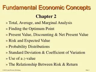
Fundamental Economic Concepts • Demand, Supply, and Equilibrium • Total, Average, and Marginal Analysis • Finding the Optimum Point • Present Value, Discounting & Net Present Value • Risk and Expected Value • Probability Distributions • Standard Deviation & Coefficient of Variation • Normal Distributions and the Standard Unit • Relationship Between Risk & Return
A demand curve shows the greatest quantity of a good demanded at each price the consumers are willing to buy, holding other influences constant (ceteris paribus). Demand Curves PRICE/Q $5 20 Quantity / time unit
Sam + Diane = Market • The market demandcurve is the horizontal SUM of the individual demand curves. • The demand function includes all variables that influence demand. 4 3 7 Q = f( P, Ps, Pc,I, N, Pe) - + - ? + + P is price of the good PS is the price of substitute goods PC is the price of complementary goods I is income, N is population, Pe is the expected future price
i. price, P ii. price of substitute goods, Ps iii. price of complementary goods, Pc iv. income, I v. advertising, A vi. advertising by competitors, Ac vii. size of population, N, viii. expected future prices, Pe xi. adjustment time period, Ta x. taxes or subsidies, T/S The list of variables that could likely affect demand varies for different industries and products. The ones on the left tend to be significant. Determinants of Demand
Supply Curves PRICE/Q • A firm’s supply curve is the greatest quantity of a good supplied at each price by the firm, holding other things constant. Quantity / time unit
Acme Inc. + Universal Ltd. = Market • The market supply curve is the horizontal sum of the firm supply curves. • The supply function includes all variables that influence supply. 4 3 7 Q = g( P, PI, RC, Tech,T/S) + - - + ?
Determinants of Supply i. price, P ii. input prices, PI (sometime shown as w (wages) and r (cost of capital) iii. cost of regulatory compliance, RC iv. expected future price, PE v. technological improvements, Tech vi. taxes or subsidies, T/S Note: Anything that shifts supply can be included and varies for different industries or products.
Dynamics of Supply and Demand • If quantity demanded is greater than quantity supplied at a price (excess demand), prices tend to rise. • The larger is the difference between quantity supplied and demanded at a price, the greater is the pressure for prices to change. • When the quantity demanded and supplied at a price are equal at a price, prices have no tendency to change.
Equilibrium: No Tendency to Change S P • Superimpose demand and supply • If no excess demand and no excess supply, then there is no tendency to change at the equilibrium price, Pe. Willing & Able in cross- hatched Pe D Q
Equilibrium Price Movements P • Suppose there is an increase in income this year and assume the good is a “normal” good • Does Demand or Supply Shift? • Suppose wages rose, what then? S P1 E1 D Q
Comparative Statics& the supply-demand model P • Suppose that demand shifts to D’ • We expect prices to rise • We expect quantity to rise as well S E2 D’ E1 D Q
Break Decisions Into Smaller Units: How Much to Produce ? profit • Graph of output and profit • Possible Rule: • Expand output until profits turn down • But problem of local maxima vs. global maximum Global MAX Local MAX A quantity B
Average Profit = Profit () / Q PROFITS • Slope of ray from the origin • Rise / Run • Profit / Q = average profit • Maximizing average profit doesn’t maximize total profit ! MAX C B profits quantity Q
Marginal Profits = /Q max profits • Q1 is breakeven (zero profit) • Maximum marginal profits occur at the inflection point (Q2) • Max average profit at Q3 • Max total profit at Q4 where marginal profit is zero • So the best place to produce is where marginal profits = 0. Q4 Q3 Q2 Q1 Q average profits marginal profits Q
Present Value • Present value recognizes that money received in the future is worth less than money in hand today. • To compare monies in the future with today, the future dollars must be discounted by a present value interest factor, PVIF=1/(1+i), where i is the interest compensation for postponing receiving cash one period. • For dollars received in n periods, the discount factor is PVIFn =[1/(1+i)]n
Net Present Value (NPV) • Most business decisions are long term. • capital budgeting, product assortment, etc. • Objective: Maximize the present value of profits • NPV = PV of future returns less initial outlay • NPV = Σt=0 NCFt / ( 1 + rt )t where NCFt is the net cash flow in period t • NPV Rule: Do all projects that have positive net present values. By doing this, the manager maximizes shareholder wealth. • Good projects tend to have: • high expected future net cash flows • low initial outlays • low rates of discount
Sources of Positive NPVs • Brand preferences for established brands • Ownership control over distribution • Patent control over products or techniques • Exclusive ownership over natural resources • Inability of new firms to acquire factors of production • Superior access to financial resources • Economies of large scale or size from either: - Capital intensive processes, or - High start up costs
Risk • Most decisions involve a gamble. • Probabilities and outcomes can be known or unknown. • We speak of risk when possible outcomes and probabilities are known. • Example is a roulette wheel or dice • We generally know the probabilities • We generally know the payouts
Concepts of Risk • When probabilities are known, we can analyze risk using probability distributions • Assign a probability to each state of nature, and be exhaustive, so that Σpi = 1 States of Nature StrategyRecessionEconomic Boom p = .30p = .70 Expand Plant- 40 100 Don’t Expand - 10 50
Payoff Matrix • Payoff Matrix shows payoffs for each state of nature, for each strategy • Expected value = r = Σ ri pi • r = Σ ri pi = (-40)(.30) + (100)(.70) = 58 if expand • r = Σ ri pi = (-10)(.30) + (50)(.70) = 32 if don’t expand • Standard deviation = = (ri - r ) 2. pi
expand = SQRT{ (-40 - 58)2(.3) + (100-58)2(.7)} = SQRT{(-98)2(.3)+(42)2 (.7)} = SQRT{ 4116} =64.16 don’t = SQRT{(-10 - 32)2 (.3)+(50 - 32)2 (.7)} = SQRT{(-42)2 (.3)+(18)2 (.7) } = SQRT{ 756 } = 27.50 In this example, expanding has a greater standard deviation (64.16) but also has the higher expected return (58). Example of Finding Standard Deviations
Coefficients of Variation or Relative Risk _ • Coefficient of variation (C.V.) = / r. • C.V. is a measure of risk per dollar of expected return. • The discount rate for present values depends on the risk class of the investment. • Look at similar investments • Corporate Bonds, or Treasury Bonds • Common Domestic Stocks, or Foreign Stocks
Projects of Different Sizes: • Coefficient of variation is a good measure for comparing projects of different sizes. • In the example below, even if size is doubled, C.V. is unchanged. Example of Two Gambles A: Prob X } R = 15 .5 10 } = SQRT{(10-15)2(.5)+(20-15)2(.5)] .5 20 } = SQRT{25} = 5 C.V. = 5 / 15 = .333 B: Prob X } R = 30 .5 20 } = SQRT{(20-30)2 ((.5)+(40-30)2(.5)] .5 40 } = SQRT{100} = 10 C.V. = 10 / 30 = .333
What Went Wrong at LTCM? • Long Term Capital Management was a ‘hedge fund’ run by some top-notch finance experts (1993-1998) • LTCM looked for small pricing deviations between interest rates and derivatives, such as bond futures. • They earned 45% returns, but that may be due to high risks in their type of arbitrage activity. • The Russian default in 1998 changed the risk level of government debt, and LTCM lost $2 billion
Normal Distributions and z-Values • z is the number of standard deviations away from the mean • z = (r - r )/σ • 68.26% of the time within 1 standard deviation • 95.44% of the time within 2 standard deviations • 99.74% of the time within 3 standard deviations Problem: income has a mean of $1,000 and a standard deviation of $500. What’s the chance of losing money? _
The Relationship of Risk & Return • Typically markets demonstrate that there is a trade-off between risk & return. • Everyone likes high returns • Many find risk something that they would like to avoid • Therefore, the market sets the premium an investor needs to accept a type of risk. • Required Return = Risk-free return + Risk Premium • In Table 2.10, if T-bills reflect the risk-free rate, on average that is 3.9%. • If large company stocks earn on average 12.7%, then the risk premium for this form of investment would be: 8.8% • 12.7% = 3.9% + 8.8% • The risk premium for other classes of assets. There would be lower risk premium for bonds and a much higher one for small company stocks.