Download
1 / 28
280 likes | 297 Views
Explore a study on pricing strategies in wireless networks, focusing on revenue maximization, social welfare, and profit balancing. Learn about two pricing strategies, Stochastic Greedy Pricing (SGP) and Bang-Bang Pricing (BB), and their impact on network efficiency and fairness.

E N D
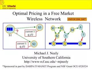
6 S1 S3 S4 current $: current $: 7 S2 5 Optimal Pricing in a Free Market Wireless Network INFOCOM 2007 S3 ? q3(t) S1 S2 q2(t) Michael J. Neely University of Southern California http://www-rcf.usc.edu/~mjneely *Sponsored in part by DARPA IT-MANET Program and NSF Grant OCE 0520324
S3 ? q3(t) S1 S2 q2(t) 6 S1 S3 S4 current $: current $: 7 S2 5 Time-slotted System: t {0, 1, 2, …} Time-Varying Channels: (fading, mobility, etc.) Sn(t) = (Sn1(t), Sn2(t), …, Snk(t)) (channel states on outgoing links of node n) Transmission Rate Options (nodes use orthogonal channels): mn(t) = (mn1(t), mn2(t), …, mnk(t)) Wn(Sn(t))
S3 ? q3(t) S1 S2 q2(t) 6 S1 S3 S4 current $: current $: 7 S2 5 Transmission Costs: Cntran(mn(t), Sn(t)) Example: Reception Costs: Cnbrec(mnb(t)) *Example: Cnbrec(mnb(t)) = { sb if mnb(t) > 0 { 0 if mnb(t) = 0 Cntran(m) m *this example is used in slides for simplicity
S3 ? q3(t) S1 S2 q2(t) 6 S1 S3 S4 current $: current $: 7 S2 5 For simplicity of these slides: Assume single commodity (multi- source, single sink) (multi-commodity case treated in the paper) Un(t) = Queue Backlog in node n at time t Rn(t) = *New data admitted to network at source n at time t New source data R2(t) Transmit out U3(t) Endogenous arrivals Node 3 (a source) *Not all nodes are sources: Some simply act as profit-seeking relays
current $: current $: S3 6 S1 S3 S4 ? q3(t) 7 S1 S2 5 S2 q2(t) For simplicity of these slides: Assume single commodity (multi- source, single sink) (multi-commodity case treated in the paper) Un(t) = Queue Backlog in node n at time t Rn(t) = *New data admitted to network at source n at time t Transmit out U5(t) Endogenous arrivals Node 5 (pure relay: not a source) *Not all nodes are sources: Some simply act as profit-seeking relays
Free Market Network Pricing: revenue Data that node n already needs to deliver Advertisement current $: qn(t) expenses rec. cost: sn Node n -Each node n sets its ownper-unit price qn(t) for accepting endogenous data from others. (Seller Node Challenge: How to set the price?) -Node n advertises qn(t)and the reception cost. (fixed reception cost sb used in slides for simplicity)
Advertisement Advertisement $ = qn(t) $ = qn(t) Buyer Node a Perspective Seller Node n Perspective rec = sn rec = sn Free Market Network Pricing: Node n Node a Advertisement $ = qn(t) rec = sn ? ? ? ? n b “Buyer Nodes” pay handling charge + reception fee: -Handling Charge: ban(t) = man(t)qn(t) -Reception Fee: sn
Advertisement Advertisement $ = qn(t) $ = qn(t) Buyer Node a Perspective Seller Node n Perspective rec = sn rec = sn Free Market Network Pricing: Node n Node a Advertisement $ = qn(t) rec = sn ? ? ? ? n b Buyer Node Challenge: Where to send? How much to send? Is advertised price acceptable? (current transmission costs Cntran(mn(t), Sn(t)) play a role, as does the previous revenue earned for accepting data)
Free Market Network Pricing: The sources’ desire for communication is the driving economic force! Modeling the Source Demand Functions: -Elastic Sources -Utility gn(r) = Source n “satisfaction” (in dollars) for sending at rate r bits/slot. h gn(r) Assumed to be: 1. Convex 2. Non-Decreasing 3. Max slope h r
Node n profit (on slot t): fn(t) = total income(t) - total cost(t) - payments(t) Source (at node n) profit (on slot t): yn(t) = gn(Rn(t)) - qn(t)Rn(t) Node n Income Payments Costs Rn(t) $ = qn(t) Source at n Node n
costn rn Social Welfare Definition: [gn( rn ) - costn ] Social Welfare = n where: = time avg admit rate from source n = time avg external costs expended by node n (not payment oriented) Simple Lemma: Maximizing Social Welfare… …is equivalent to maximizing sum profit (sum profit = “network GDP”) (ii)…can (in principle) be achieved by a stationary randomized routing and scheduling policy
We will design 2 different pricing strategies: Stochastic Greedy Pricing (SGP): - Greedy Interpretation - Guarantees Non-Negative Profit - If everyone uses SGP, Social Welfare Maxed over all alternatives (and so Sum Profit Maxed) 2) Bang-Bang Pricing (BB): - No Greedy Interpretation - Yields a “optimally balanced” profits (profit fairness…minimizes exploitation)
Prior Work: Utility Maximization for Static Networks: [Kelly: Eur. Trans. Tel. 97] [Kelly, Maulloo, Tan: J. Oper. Res. 98] [Low, Lapsley: TON 1999] [Lee, Mazumdar, Shroff: INFOCOM 2002] Utility Maximization for Stochastic Networks: [Neely, Modiano, Li: INFOCOM 2005] [Andrews: INFOCOM 2005] [Georgiadis, Neely, Tassiulas: NOW F&T 2006] [Chen, Low, Chiang, Doyle: INFOCOM 2006] Pricing plays only an indirect role in yielding max utility solution For the stochastic algorithms, dynamic “prices” do not necessarily yield the non-negative profit goal!
Prior Work: Revenue Maximization for Downlinks (non-convex): [Acemoglu, Ozdaglar: CDC 2004] [Marbach, Berry: INFOCOM 2002] [Basar, Srikant: INFOCOM 2002] Markov Decision Problems for single-network owner: [Paschalidis, Tsitsiklis TON 2000] [Lin, Shroff TON 2005] Market Mechanisms: [Buttyan, Hubaux: MONET 2003] [Crowcroft, Gibbens, Kelly, Ostring WiOpt 2003] [Shang, Dick, Jha: Trans. Mob. Comput. 2004] [Marbach, Qui: TON 2005] Profit is central to problem Need a stochastic theory for market-based network economics!
qn(t) = Un(t)/V Stochastic Greedy Pricing Algorithm (SGP): (Similar to Cross-Layer-Control (CLC) Algorithm from [Neely 2003] [Neely, Modiano, Li INFOCOM 2005]) For a given Control Parameter V>0… Pricing (SGP): Rn(t) Node n Admission Control (SGP): “instant utility” payment Queue Backlog Un(t) Max: gn(Rn(t)) - qn(t) Rn(t) Subj. to: 0 < Rn(t) < Rmax
Stochastic Greedy Pricing Algorithm (SGP): (Similar to Cross-Layer-Control (CLC) Algorithm from [Neely 2003] [Neely, Modiano, Li INFOCOM 2005]) For a given Control Parameter V>0… Resource Allocation & Routing (SGP): Define the modified differential price Wnb(t): Wnb(t) = qn(t) - qb(t) - d/V qn(t) qb(t) where d = max[mmax out, mmax in + Rmax] Maximize: Wnb(t)mnb(t) - Cnbrec(mn(t)) - Cntran(mn(t), Sn(t)) Subj. to : mn(t) Wn(Sn(t)) b b
t-1 t-1 > 0 qn(t) Rn(t) Rn(t) t-1 t=0 t=0 1 1 1 gn( ) - fn(t) > 0 t t t t=0 Theorem (SGP Performance): For arbitrary S(t) processes and for any fixed parameter V>0: Un(t) < Vh + d for all n, for all time t All nodes and sources receive non-negative profit at every instant of time t: Nodes: Sources: (a)(b) hold for any node n using SGP, even if others don’t use SGP!
Theorem (SGP Performance): For arbitrary S(t) processes and for any fixed parameter V>0: Un(t) < Vh + d for all n, for all time t All nodes and sources receive non-negative profit at every instant of time t: (c) If Channel States S(t) are i.i.d. over slots and if everyone uses SGP: Social Welfare > g* - O(1/V) g* = maximum social welfare (sum profit) possible, optimized over all alternative algorithms for joint pricing, routing, resource allocation.
Simulation of SGP: 6 S1 S3 S4 7 S2 5 Parameters: V= 50 Dotted Links: ON/OFF Channels (Pr[ON] = 1/2) Transmission costs = 1 cent/packet, reception costs = .5 cent/packet Solid Links: Transmission costs = 1 cent/packet Utilities: g(r) = 10 log(1 + r)
6 SGP: V=50 C2 = C5 = C7 = 1 g(r) = 10 log(1+r) S1 S3 S4 7 S2 5 Simulation of SGP:
6 SGP: V=50 C7=1 C2 = C5 = 3 g(r) = 10 log(1+r) S1 S3 S4 7 S2 5 Simulation of SGP (increase cost of C2, C5):
[ Fn( fn ) + Yn( yn ) ] n Bang-Bang Pricing (BB) Algorithm: Objective is to Maximize: Where Fn(f) and Yn(y) are concave profit metrics. Yields a more balanced (and “fair”) profit distribution.
Quick (incomplete) description of Bang-Bang Pricing (see paper for details):Uses General Utility Optimization technique from our previous work in [Georgiadis, Neely, Tassiulas NOW F & T 2006] BB Algorithm: Define Virtual Queues Xn(t), Yn(t) And Auxiliary Variablesgn(t), nn(t). income(t) expenses(t) + gn(t) Nodes n: Xn(t) gn(Rn(t)) payment(t) + nn(t) Sources n: Yn(t)
Pricing (BB): qan(t) = { Qmax if Xa(t) < Xn(t) { 0 else (Price depends on the incoming link) Distributed Auxiliary Variable Update: Each node n solves: Maximize: VFn(g) - Xn(t)g Subject to: 0 < g < Qmax d Resource Allocation Based on Mod. Diff. Backlog: Wnb(t) = Un(t) - Ub(t) -qnb(t)[Xn(t) - Xb(t)]
[ Fn( fn ) + Yn( yn ) ] n > Optimal - O(1/V) Theorem (BB Performance): If all nodes Use BB with parameter V>0, then: 1) Avg. Queue Congesetion < O(V) 2)
6 SGP: V=50 C2 = C5 = C7 = 1 g(r) = 10 log(1+r) S1 S3 S4 7 S2 5 Simulation of BB:
6 SGP: V=50 C7=1 C2 = C5 = 3 g(r) = 10 log(1+r) S1 S3 S4 7 S2 5 Simulation of BB (increase cost of C2, C5):
6 SGP: V=50 C7=1 C2 = C5 = 3 g(r) = 10 log(1+r) S1 S3 S4 7 S2 5 Conclusions: SGP: Guarantees Non-negative profit and Bounded queues, Regardless of actions of Other nodes. If all nodes Use SGP => Max sum Profit! 2) BB: Optimally Balanced, but has no greedy interpretation.