Download
1 / 48
480 likes | 557 Views
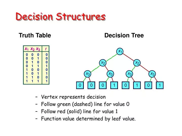
Decision Structures. Vertex represents decision Follow green (dashed) line for value 0 Follow red (solid) line for value 1 Function value determined by leaf value. Truth Table. Decision Tree. Variable Ordering. Assign arbitrary total ordering to variables e.g., x 1 < x 2 < x 3

E N D
Decision Structures • Vertex represents decision • Follow green (dashed) line for value 0 • Follow red (solid) line for value 1 • Function value determined by leaf value. Truth Table Decision Tree
Variable Ordering • Assign arbitrary total ordering to variables • e.g., x1 < x2 < x3 • Variables must appear in ascending order along all paths OK Not OK Properties • No conflicting variable assignments along path • Simplifies manipulation
a a a Reduction Rule #1 Merge equivalent leaves
x x x x x x y z y z y z Reduction Rule #2 Merge isomorphic nodes
x y y Reduction Rule #3 Eliminate Redundant Tests
Example OBDD Initial Graph Reduced Graph • Canonical representation of Boolean function • For given variable ordering • Two functions equivalent if and only if graphs isomorphic • Can be tested in linear time • Desirable property: simplest form is canonical.
Constants Variable Unique unsatisfiable function Treat variable as function Unique tautology Typical Function Odd Parity • (x1 x2 ) x4 • No vertex labeled x3 • independent of x3 • Many subgraphs shared Linear representation Example Functions
Representing Circuit Functions • Functions • All outputs of 4-bit adder • Functions of data inputs • Shared Representation • Graph with multiple roots • 31 nodes for 4-bit adder • 571 nodes for 64-bit adder • Linear growth
Linear Growth Exponential Growth Effect of Variable Ordering Good Ordering Bad Ordering
Bit Serial Computer Analogy • Operation • Read inputs in sequence; produce 0 or 1 as function value. • Store information about previous inputs to correctly deduce function value from remaining inputs. • Relation to OBDD Size • Processor requires K bits of memory at step i. • OBDD has ~ 2K branches crossing level i.
K = 2 K = n Analysis of Ordering Examples
Selecting Good Variable Ordering • Intractable Problem • Even when problem represented as OBDD • I.e., to find optimum improvement to current ordering • Application-Based Heuristics • Exploit characteristics of application • E.g., Ordering for functions of combinational circuit • Traverse circuit graph depth-first from outputs to inputs • Assign variables to primary inputs in order encountered
Dynamic Variable Reordering • Richard Rudell, Synopsys • Periodically Attempt to Improve Ordering for All BDDs • Part of garbage collection • Move each variable through ordering to find its best location • Has Proved Very Successful • Time consuming but effective • Especially for sequential circuit analysis
Best Choices Dynamic Reordering By Sifting • Choose candidate variable • Try all positions in variable ordering • Repeatedly swap with adjacent variable • Move to best position found • • •
g h i j e f g h b b b b b b b b 1 1 1 1 2 2 2 2 i j f e b b b b 1 1 2 2 Swapping Adjacent Variables • Localized Effect • Add / delete / alter only nodes labeled by swapping variables • Do not change any incoming pointers
Sample Function Classes Function Class Best Worst Ordering Sensitivity ALU (Add/Sub) linear exponential High Symmetric linear quadratic None Multiplication exponential exponential Low • General Experience • Many tasks have reasonable OBDD representations • Algorithms remain practical for up to 100,000 node OBDDs • Heuristic ordering methods generally satisfactory
• • • • • • • • • • • • Lower Bound for Multiplication bn-1 p2n-1 Multn Intractable Function • Bryant, 1991 • Integer Multiplier Circuit • n-bit input words A and B • 2n-bit output word P • Boolean function • Middle bit (n-1) of product • Complexity • Exponential OBDD for all possible variable orderings b0 pn an-1 pn-1 a0 p0 Actual Numbers • 40,563,945 BDD nodes to represent all outputs of 16-bit multiplier • Grows 2.86x per bit of word size
Symbolic Manipulation with OBDDs • Strategy • Represent data as set of OBDDs • Identical variable orderings • Express solution method as sequence of symbolic operations • Implement each operation by OBDD manipulation • Algorithmic Properties • Arguments are OBDDs with identical variable orderings. • Result is OBDD with same ordering. • “Closure Property” • Contrast to Traditional Approaches • Apply search algorithm directly to problem representation • E.g., search for satisfying truth assignment to Boolean expression.
If-Then-Else Operation • Concept • Basic technique for building OBDD from logic network or formula. Arguments I, T, E • Functions over variables X • Represented as OBDDs Result • OBDD representing composite function • (I T)(I E) Implementation • Combination of depth-first traversal and dynamic programming. • Worst case complexity product of argument graph sizes.
Recursive Calls If-Then-Else Execution Example Argument I Argument T Argument E • Optimizations • Dynamic programming • Early termination rules
If-Then-Else Result Generation Recursive Calls Without Reduction With Reduction • Recursive calling structure implicitly defines unreduced BDD • Apply reduction rules bottom-up as return from recursive calls • Generates reduced graph
Restriction Operation • Concept • Effect of setting function argument xi to constant k (0 or 1). • Also called Cofactor operation (UCB) Implementation • Depth-first traversal. • Complexity near-linear in argument graph size
Derived Operations • Express as combination of If-Then-Else and Restrict • Preserve closure property • Result is an OBDD with the right variable ordering • Polynomial complexity • Although can sometimes improve with special implementations
Derived Algebraic Operations • Other operations can be expressed in terms of If-Then-Else If-Then-Else(F, G, 0) And(F, G) If-Then-Else(F, 1, G) Or(F, G)
Functional Composition • Create new function by composing functions F and G. • Useful for composing hierarchical modules.
Variable Quantification • Eliminate dependency on some argument through quantification • Combine with AND for universal quantification.
Digital Applications of BDDs • Verification • Combinational equivalence (UCB, Fujitsu, Synopsys, …) • FSM equivalence (Bull, UCB, MCC, Siemens, Colorado, Torino, …) • Symbolic Simulation (CMU, Utah) • Symbolic Model Checking (CMU, Bull, Motorola, …) • Synthesis • Don’t care set representation (UCB, Fujitsu, …) • State minimization (UCB) • Sum-of-Products minimization (UCB, Synopsys, NTT) • Test • False path identification (TI)
Generating OBDD from Network Task:Represent output functions of gate network as OBDDs. • A new_var ("a"); • B new_var ("b"); • C new_var ("c"); • T1 And (A, 0, B); • T2 And (B, C); • Out Or (T1, T2); Network Evaluation Resulting Graphs
a b b a b c c c 0 1 0 1 0 1 Checking Network Equivalence Task: Do two networks compute same Boolean function? Method: Compute OBDDs for both networks and compare Alternate Network Evaluation T1 Or (A, C); O2 And (T1, B); if (O2 == Out) then Equivalent else Different O2 Resulting Graphs T1 A B C a 0 1 0 1
Finite State System Analysis • Systems Represented as Finite State Machines • Sequential circuits • Communication protocols • Synchronization programs • Analysis Tasks • State reachability • State machine comparison • Temporal logic model checking • Traditional Methods Impractical for Large Machines • Polynomial in number of states • Number of states exponential in number of state variables. • Example: single 32-bit register has 4,294,967,296 states!
Union Intersection Characteristic Functions • Concept • A {0,1}n • Set of bit vectors of length n • Represent set A as Boolean function A of n variables • XA if and only if A(X ) = 1 Set Operations
00 01 o 1 o o 2 2 10 11 n 1 n 2 0 1 Symbolic FSM Representation Symbolic Representation Nondeterministic FSM • Represent set of transitions as function (Old, New) • Yields 1 if can have transition from state Old to state New • Represent as Boolean function • Over variables encoding states o , o encoded 1 2 old state n , n encoded 1 2 new state
old state new state Reachability Analysis • Task • Compute set of states reachable from initial state Q0 • Represent as Boolean function R(S) • Never enumerate states explicitly Given Compute d 0/1 Initial
R1 R1 R1 R0 R2 R2 R0 R0 R0 01 01 01 10 10 00 01 00 00 00 00 10 11 R3 Breadth-First Reachability Analysis • Ri – set of states that can be reached initransitions • Reach fixed point when Rn = Rn+1 • Guaranteed since finite state
R i +1 R i $ old d new R i Iterative Computation • Ri +1 – set of states that can be reachedi +1 transitions • Either in Ri • or single transition away from some element of Ri
R0 01 o 1 00 o o 2 2 Old [R0(Old) (Old, New)] n n n n 1 1 1 1 n n n 2 2 2 0 0 0 0 0 0 1 1 1 1 R1 00 Example: Computing R1 from R0
Symbolic FSM Analysis Example • K. McMillan, E. Clarke (CMU) J. Schwalbe (Encore Computer) • Encore Gigamax Cache System • Distributed memory multiprocessor • Cache system to improve access time • Complex hardware and synchronization protocol. • Verification • Create “simplified” finite state model of system (109 states!) • Verify properties about set of reachable states • Bug Detected • Sequence of 13 bus events leading to deadlock • With random simulations, would require 2 years to generate failing case. • In real system, would yield MTBF < 1 day.
What’s Good about OBDDs • Powerful Operations • Creating, manipulating, testing • Each step polynomial complexity • Graceful degradation • Maintain “closure” property • Each operation produces form suitable for further operations • Generally Stay Small Enough • Especially for digital circuit applications • Given good choice of variable ordering • Weak Competition • No other method comes close in overall strength • Especially with quantification operations
What’s Not Good about OBDDs • Doesn’t Solve All Problems • Can’t do much with multipliers • Some problems just too big • Weak for search problems • Must be Careful • Choose good variable ordering • Critical effect on efficiency • Must have insights into problem characteristics • Dynamic reordering most promising workaround • Some operations too hard • Must work around limitations
Relaxing Ordering Requirement • Challenge • Ordering is key to important properties of OBDDs • Canonical form • Efficient algorithms for operating on functions • Some classes of functions have no good BDD orderings • Graphs grow exponentially in all cases • Would like to relax requirement • but still preserve (most of) the algorithmic properties • Free Ordering • Gergov & Meinel, Sieling & Wegener • Slight relaxation of ordering requirement
Control Data Rotate Difficult Function • Rotate & compare Rotations 0 1 C 2 3 Rotate A = B Intractable OBDD Function Example • Rotator • Circular shift of data • Shift amount set by control
Can choose good ordering for any fixed rotation OBDDs for Specific Rotations
Forcing Single Ordering • Good ordering for one rotation terrible for another • For any ordering, some rotation will have exponential OBDD
Free BDDs • Rules • Variables may appear in any order • Only allowed to test variable once along any path Not OK OK Extraneous path
Rotation Function Example • Advantage • Can select separate ordering for each rotation • Good when different settings of control call for different orderings of data variables • Still Has Limitations • Representing output functions of multiplier • Exponential for all possible Free BDDs • Ponzio, ‘95
Making Free BDDs Canonical • Modified Ordering Requirement • For any given variable assignment, variables must occur in fixed order • But can vary from one assignment to another • Algorithmic Properties Similar to OBDDs • Reduce to canonical form • Apply Boolean operation to functions • Test for equivalence, satisfiability, etc. • Some Operations Harder • Variable quantification and composition • But can restrict relevant variables to be totally ordered
Representing Free Ordering • Ordering Graph • Encodes assignment-dependent variable ordering • Similar to BDD • Follow path according to assignment • OBDD is Special Case • Linear chain • Ordering Requirement • All functions must be compatible with single ordering graph
Practical Aspects of Free BDDs • Make Sense in Some Application Domain • Usage of bits varies with context • E.g., instruction set encodings • Must Determine Good Ordering Graph • Some success with heuristic methods • Ideally should be done dynamically • Overwhelming degrees of freedom • Need to Demonstrate Utility on Real-Life Examples