Download
1 / 30
300 likes | 538 Views
Possible disk emission in the BLR of AGN. E di Bon Astronomical Observatory Belgrade, Serbia ebon@aob.bg.ac.yu L. Č. Popović 1 , D . I lić 2 1- Astronomical Observatory Belgrade, Serbia 2- University of Belgrade, Faculty of Mathematics Department of Astronomy. Intro:.

E N D
Possible disk emission in the BLR of AGN Edi Bon Astronomical Observatory Belgrade, Serbia ebon@aob.bg.ac.yu L. Č. Popović1 , D. Ilić2 1- Astronomical Observatory Belgrade, Serbia 2- University of Belgrade, Faculty of Mathematics Department of Astronomy
Intro: I – Here we investigated the structure of broad emission profiles (Hα, Hβ…) II – To explain the structure of these profiles we simplified the things using “two-component model”, with assumption that the wings of the lines originated in the disk, and a spherical region that surrounds the disk contributes to the core of the lines. III – we applied this model to the profiles of 14 single-peaked AGN (that we observed at INT), that already had a proof of the disk existence in X domain of spectra IV – the fitting to this model allowed as to do only ruff estimation of parameters, because of luck of shoulders or bumps and the large number of parameters of our model V – in order to determine better fit, we simulated our model for different parameters so we could estimate influence of the disk flux in the profiles
0 Unification Scheme of AGN
0 Grand Unification Scheme
0 Grand Unification Scheme
masers BLR Torus BAL 0 Unification Scheme of AGN Emmering, Blandford & Shlosman 1992 • Torus – samo oblast u vetru akrecionog diska
I(l)=IAD(l)+IG(l) Two-component model Where: IAD(l)the emissions of the relativistic accretion disk IG(l)the emissions of the spherical region around the disk • The disk is contributing to the wings of the lines, • a spherical medium arround the disk to the core of the lines. The whole line profile can be described by the relation:
Disk model Chen & Halpern (1989).
Sl. 1: Dekompozicija Hβ linijeposmatrana na INT-u. Isprekidana linija pretstavlja posmatranja,dok puna linija pretstavlja najbolji fit. Na dnu su gausove komponente i isprekidana linija koja pretstavlja doprinos Fe II multipleksa
Sl. 2: Isto kao Sl. 1, samo za Hα liniju. Pored uske Hα centralne komponente, prisutne su dve slabe uske [NII] linije: na 7136 Å i 7174 Å
Fit IIIZw2 • the comparison of all line profiles (dashed lines) with an averaged one (solid line); • fit of the averaged line profile. c),d),e),f) represent fit of Lyα, Mg II, Hβ and H α lines, resp.
MODEL IIIZw2 zdisk – shift of the disk komponents– width of Gaussianin the diskRinninner radiusRoutouter radiuszGshift of the GaussianWGwidth of the Gaussian< AV >averaged prfileFD/FGflux ratio
Two fits of 3C 273 with the two-component model the disk parameters are: a) i=14°, Rinn=400 Rg, Rout=1420 Rg, Wd=1620 km/s, p=3.0 (WG=1350 km/s); b) i=29°, Rinn=1250 Rg, Rout=15000 Rg, Wd=700 km/s, p=2.8 (WG=1380 km/s)
The random velocities of a spherical region (ILR) as a function of the local random disk velocities. The dashed line represents the function VILR = VDisk [km s−1].
Gaussian flux = 1/2 disk flux Ratio of FWHM& width@10-40% of hight in function of inclination. over25% disk is weak
Gaussian flux = 1/3 disk flux Ratio of FWHM& width@5-45% of hight in function of inclination. over40% disk is weak
Gaussian flux = 3 x disk flux Ratio of FWHM& width@2-30% of hight in function of inclination. over 10% disk is weak
Gaussian flux = 2 x disk flux Ratio of FWHM& width@5-35% of hight in function of inclination. over 10-15% disk is not detectable.
Gaussian flux= disk flux Ratio of FWHM& width@ 3-30%.
Gaussianflux = diskflux, for inclinationi=30, Fixed ring, width 800, Rinn from 200 to 1200
Gaussianflux = diskflux, for inclinationi=30, Weith response to emisivity
Gaussianflux = diskflux, for inclinationi=20, Fixed ring, width 800, Rinn from 200 to 1200
Wx/W50 3c120 10 % - 2.867891 20 % - 1.915054 Height [%]
na 10% fori=20 2.9=> Rinn=600 na 20% for i=20 1.9=> Rinn=1000 --------------------------------------------------------------- Flux of Gaussian = 1/2 fluks of disk 10% 2.9=> i=20 20% 2=>i=25 Flux of Gaussian = 1/3 fluks of disk 10% 2.9 =>i=26 20% 1.9=> i=25 Flux of Gaussian = 3 x fluks of disk 10% 3 => i=15 20% 1.65=>i=15 max Flux of Gaussian = fluks of disk 10% 2.8 => i=15 20% 1.9=> i=12 Flux of Gaussian = 2 x fluks of disk 10% 2.6 =>i=15 20% 1.75 => i=20 max 3c12010 %: 2.867891 20 %: 1.915054
na 10% za i=10 2.9=> Rinn=170 na 20% za i=10 1.9=> Rinn=230 na 10% za i=122.9=> Rinn=200 na 20% za i=121.9=> Rinn=250 na 10% za i=152.9=> Rinn=320 na 20% za i=151.9=> Rinn=600
Future work: • To simulate for finer grid of inclinations and rings • To apply for large number of real spectra of AGN • To analyze expectations of the disk influence in the fluxes of emission line profiles of the AGN spectra • ...